5 Statistical inference
This is the published R edition of the book. A Python version of the book is available at era_pl_book.
In this chapter, we study statistical inference in the context of null hypothesis significance testing (NHST), which is the predominant paradigm in empirical accounting research. We examine NHST in fairly procedural terms without spending too much time justifying it. One reason for doing so is that, even if we simply accept NHST as a sensible approach to science, the way NHST is used in practice is profoundly different from how it was expected to be used when its epistemological foundations were set.1 So real problems with NHST exist long before reaching those foundations.
Another issue with NHST is that statistical inference in most settings is based on limit theorems—results from mathematical statistics that can require fairly advanced mathematics to prove—such as laws of large numbers and central limit theorems.2 To minimize the mathematical requirements here, we use simulations to illustrate ideas rather than trying to provide mathematically precise results. For readers looking to go deeper on either dimension, we provide a guide to further reading at the end of the chapter.
The code in this chapter uses the packages listed below. For instructions on how to set up your computer to use the code found in this book, see Section 1.2 (note that Step 4 is not required as we do not use WRDS data in this chapter). Quarto templates for the exercises below are available on GitHub.
5.1 Some observations
Students of econometrics in PhD programs often spend much of their time learning about the asymptotic properties of estimators, which might be understood as describing how estimators behave as sample sizes tend towards infinity. However, there are two gaps in this pedagogical approach. First, it is often not made clear why we care about asymptotic properties of estimators. A practical student might question the relevance of asymptotic properties when sample sizes in practice can at times be quite large, but are rarely infinite.
Second, in practice, researchers soon forget that the estimators they use are justified by their asymptotic properties and rarely exploit what they learned in econometrics classes to study new estimators. For example, in this chapter we will devote some time to the study of standard errors. Almost all estimators of standard errors are motivated by asymptotic properties and thus can perform poorly in actual research settings. Yet Gow et al. (2010) show that estimators can gain currency among researchers without any formal analysis of their properties, asymptotic or otherwise.
One reason for studying the asymptotic properties of estimators is that they are mathematically tractable for a well-trained econometrician. For a practical researcher, knowing that an estimator has good asymptotic properties might be considered more or less necessary. An estimator that is not consistent is apt to produce significantly biased estimates in finite samples (one can think of consistency as the asymptotic equivalent of unbiasedness).3 And good asymptotic properties might be practically sufficient for the estimator to behave well in finite samples. An estimator that is asymptotically efficient and asymptotically normal might have a good chance of being an efficient estimator in finite samples and having a distribution that is sufficiently close to the normal distribution for practical statistical inference.
In this chapter, we will not derive asymptotic properties of estimators. Instead, we direct readers to econometrics texts for these details. Additionally, while we provide an intuitive introduction to laws of large numbers and central limit theorems, we do not even state these formally, let alone derive them. Instead, in keeping with a theme of this book, we will use simulations to give the reader an intuitive feel for where these results from mathematical statistics come from and what they mean.
5.2 Data-generating processes
Like causal inference, thinking about statistical inference generally involves quite abstract reasoning. Before getting into the statistics, it is helpful to imagine that the data we observe are generated by an underlying process (hence a data-generating process or DGP). A DGP will often look like a model, but in principle these are distinct ideas. The DGP is a feature of reality that we generally do not observe directly, while a model is a guess or useful simplification of a conjectured DGP that humans use to understand the DGP.
In some settings, we may believe that our model captures all the essential details of the DGP. While the results of a coin toss will depend on the rotational momentum imparted to the coin, the vertical velocity of the coin, imperfections on the coin’s surface, prevailing humidity, temperature, wind velocity, and so on, we may be happy in simply using a model in which coin tosses are independent, and equally likely to be one outcome as the other.
Part of the potential for confusion between these two ideas is that when discussing a DGP, we inevitably use a model, as we do here. Suppose that the height in centimetres of adult individuals is drawn from a normal distribution with mean of \(\mu = 165\) and standard deviation of \(\sigma = 8\).
hgt_mean <- 165
hgt_sd <- 8
This statement could be interpreted as the process for generating the heights of the billions of adult people who happen to inhabit Earth at this time. In a sense, the people who actually exist are a non-deterministic sample of the potential people who could exist.4
Alternatively, we might take the current inhabitants of the world as given and posit that the empirical distribution of heights is actually a normal distribution with parameters \(\mu\) and \(\sigma\), and focus instead on taking random sample from that population. Looking ahead, we might use a random sample to make inferences about the distribution of heights of adult humans who currently inhabit the world or about the data-generating process for adult heights. In the context of causal inference, it is often the latter kind of inference that we want to make, but for present purposes, we focus on the former kind.
There is no doubt that a two-parameter normal distribution is an oversimplification of the actual DGP, hence more of a model than an actual DGP. For example, we make no allowance for heights varying around the world, for the tendency of heights to increase over time (hence the reference to “current” above), or the tendency for men to be taller than women, each of which may undermine the applicability of a simple assumed DGP. But for current purposes, we ignore such quibbles and simply assume that heights come from a normal distribution \((\mu, \sigma)\).
We can simulate the taking of a random sample of size \(n = 100\) by using the rnorm() function we saw in Chapter 2.
hgt_sample <- rnorm(100, mean = hgt_mean, sd = hgt_sd)Given that we know that \(\mu = 165\) and that \(\sigma = 8\), we can calculate expected values for the mean and standard deviation of the heights in our sample. Here the sample mean is calculated as the sum of the observed heights (\(\{x_i: i \in (1, \dots, n)\}\)) divided by \(n\), where \(n = 100\).
\[ \overline{X}_{n} = \frac{\sum_{i = 1}^{n} x_i}{n} \]
\[ \begin{aligned} \mathbb{E}[\overline{X}_{n}] &= \mathbb{E}\left[\frac{\sum_{i = 1}^{n} x_i}{n}\right] \\ &= \frac{\sum_{i = 1}^{n} \mathbb{E}\left[ x_i\right]}{n} \\ &= \frac{n \mu}{n} \\ &= \mu \end{aligned} \] To calculate the variance of \(\overline{X}_{n}\), we note that the variance of \(ax\), where \(a\) is a constant and \(x\) is a random variable, is \(\mathrm{Var}[ax] = a^2 \mathrm{Var}[x]\) and the variance of the sum of independent and identically distributed variables \(x_i\), \(i \in (1, \dots, n)\), each with variance \(\sigma^2\), is simply the sum of their variances:
\[ \begin{aligned} \mathrm{Var} \left[\sum_{i = 1}^{n} x_i \right] &= \sum_{i = 1}^{n} \mathrm{Var} \left[x_i \right] \\ &=n \sigma^2 \end{aligned} \]
The variance of \(x/k\) for some constant \(k \neq 0\) is
\[ \begin{aligned} \mathrm{Var} \left(\frac{x}{k}\right) &= \sum_{i = 1}^{n} \frac{1}{n} \left( \frac{x_i - \overline{x}}{k} \right)^2 \\ &= \frac{1}{k^2} \sum_{i = 1}^{n} \frac{1}{n} \left( x_i - \overline{x} \right)^2 \\ &= \frac{1}{k^2} \mathrm{Var} \left(x \right) \end{aligned} \] From the above, we can calculate the following:
\[ \begin{aligned} \mathrm{Var}[\overline{X}_{n}] &= \mathrm{Var} \left[\frac{\sum_{i = 1}^{n} x_i}{n}\right] \\ &= \frac{1}{n^2} \mathrm{Var} \left[\sum_{i = 1}^{n} x_i \right] \\ &= \frac{\sigma^2}{n} \end{aligned} \] The standard deviation of the sample mean is the square root of its variance: \(\frac{\sigma}{\sqrt{n}}\).
This section may seem a little bewildering on a first reading because we cover a lot of concepts in R quickly. Our recommendation is to play around with the code yourself as you work through this section and focus more on the inputs and outputs than the finer details of the code at this point.
Because in this section, we are in an idealized world in which we know the underlying DGP, we can test our calculations by generating data. We can incorporate the code we used to make a sample above in a function get_hgt_sample() that takes a single argument (n) for the sample size.
get_hgt_sample <- function(n) {
  rnorm(n, mean = hgt_mean, sd = hgt_sd)
}
Calling get_hgt_sample() with n = 10, we get a sample of 10 random numbers. We use set.seed(2023) so that we get the same random numbers each time. The value 2023 is completely arbitrary (it was the current year when we first wrote this chapter).5
set.seed(2023)

get_hgt_sample(10)
[1] 164.3297 157.1365 149.9995 163.5108 159.9321 173.7264 157.6902 173.0131
[9] 161.8059 161.2550But we can easily generate ten-thousand samples. In many programming languages, we would use a for loop to do this and R offers such functionality, as seen in the following code (Chapter 27 of R for Data Science discusses for loops). In R, it is natural to use a list to store results from multiple runs of a function, so we initialize hgt_samples as an empty list and then use the for command to repeat the get_hgt_sample(100) call 10,000 times, storing each sample in a slot in hgt_samples (we discussed lists in Chapter 2).
n_samples <- 10000
We can take a peek at the first ten observations in the 463rd sample like this:
hgt_samples[[463]][1:10] [1] 168.4070 164.0360 163.2143 155.2887 163.0420 170.6284 146.7339 168.8120
[9] 172.7608 156.1855We can calculate the mean of the 463rd sample like this:
mean(hgt_samples[[463]])[1] 164.4264We could use a for loop to calculate the mean for each of the samples in one go, storing the results in a new list, hgt_sample_means.
We can peek at the first 5 values of hgt_sample_means like this:
hgt_sample_means[1:5][[1]]
[1] 165.5401
[[2]]
[1] 166.6662
[[3]]
[1] 163.7082
[[4]]
[1] 165.0866
[[5]]
[1] 164.1906For many purposes, it will be easier to work with hgt_sample_means if it is a vector rather than a list and we can use the unlist() function to convert it to a vector:
unlist(hgt_sample_means[1:5])[1] 165.5401 166.6662 163.7082 165.0866 164.1906Additionally, we could use one of the map() functions, such as map_vec(), from the purrr library rather than a for loop. Chapter 26 of R for Data Science covers the purrr library. The map(x, f) function maps the function f() to each element of the vector x and returns a list containing the results. In our case, x will be a column of a data frame and, because we want the result of each calculation here to be a vector, we use map_vec(), which is like map() but with the output simplified to a vector.6
hgt_sample_means <- map_vec(hgt_samples, mean)We can see we have a nice vector of means from a single line of code.
hgt_sample_means[1:10] [1] 165.5401 166.6662 163.7082 165.0866 164.1906 164.9117 164.3328 164.5542
[9] 164.1957 164.8957In fact, we could have used map() rather than a for-loop to create hgt_samples in the first place.
Note that, to get n_samples samples, we want to map() the get_hgt_sample() function to the vector 1:n_samples. But we have a small problem: map() will provide each value of that vector to get_hgt_sample(), and get_hgt_sample() simply does not expect that value. One approach to addressing this is to use an anonymous function as we do below.
We call function(x) get_hgt_sample(100) an anonymous function because we do not give it a name. Note that we could also use a shortcut form that allows us to write an anonymous function(x) get_hgt_sample(100) as simply \(x) get_hgt_sample(100). While we could give the function a name (by storing it in a variable), this means creating a new variable (get_hgt_sample_alt) without producing code that is easier to read.
Another approach would be to make a version of get_hgt_sample() that does expect an argument related to the index of the sample being generated. In fact, in some settings, it might be useful to retain that information, so we have get_hgt_sample_df() return a data frame (tibble) containing the sample index in the first column (i) and the actual sample in the second column (data).
To see what get_hgt_sample_df() is doing, we call it once to get a single (small) sample.
one_sample <- get_hgt_sample_df(i = 1, n = 10)Looking at the data frame one_sample, we can see that it has two columns and only one of these—data—is a list column.
one_sample# A tibble: 1 × 2
i data
<dbl> <list>
1 1 <dbl [10]>Looking at the first value in the data column, we see that it’s a vector of ten values.
one_sample$data[[1]] [1] 159.2986 172.3488 170.3377 172.4086 161.2063 171.0710 164.7035 183.3683
[9] 152.9049 171.6578So let’s get n_samples using this approach.
While we can access the underlying data in hgt_samples, it might seem that we are adding complexity for no particular reason, especially if we compare the code for looking at the 463rd sample below to the equivalent code in our first attempt above.
unlist(hgt_samples[[463]]$data)[1:10] [1] 168.4070 164.0360 163.2143 155.2887 163.0420 170.6284 146.7339 168.8120
[9] 172.7608 156.1855One reason for this complexity is that currently hgt_samples is a list of tibbles. We can use the function list_rbind() to bind them together into a single data frame.
hgt_samples_df <- list_rbind(hgt_samples)Note that hgt_samples_df is starting to get fairly large:
print(object.size(hgt_samples_df), units = "auto")8.2 MbWhile the size of hgt_samples_df does not present a problem for a modern computer, more complicated analyses might produce objects sufficiently large that we would want to pay attention to their sizes. We can now use map_vec() to extract statistics from hgt_samples_df. To keep our results small, we then drop the data column from our table of statistics (hgt_samples_stats). (We could always use the column i to join hgt_samples_stats with hgt_samples_df if we wanted to recover these data.)
We can now assess how well our formulas worked out in our simulations. We calculate the mean and standard deviation of the means, as well as the mean of the standard errors.
# A tibble: 1 × 5
      n mean_mean sd_mean mean_se  sd_se
  <dbl>     <dbl>   <dbl>   <dbl>  <dbl>
1   100      165.   0.810   0.799 0.0569
The mean of the estimated means is indeed pretty close to the \(\mu\) parameter of 165 and the standard deviation of those estimated means is also very close to the value \(\frac{\sigma}{\sqrt{n}}\) (0.8).
We can examine the errors in our estimates using transmute(), which acts like mutate() except that transmute() does not retain columns not calculated in the function call.
# A tibble: 1 × 3
  mean_error se_error se_est_error
       <dbl>    <dbl>        <dbl>
1     0.0110  0.01000      -0.0112
5.2.1 Discussion questions
Explain what “error” each of
mean_error,se_error, andse_est_erroris capturing.What effects do you expect changes in the values of
n_samplesornto have onmean_error? Do you expect changingn_samplesor changingnto have a greater effect? Verify your conjectures using the simulation code. (Hint: Consider 100,000 draws of samples of 100 and 10,000 draws of samples of 1,000. In each case, you shouldset.seed(2023)afresh and effectively replace data inhgt_samples.)
5.3 Hypothesis testing
Of course, in reality we generally do not observe parameters like hgt_mean and hgt_sd and our task as statisticians is to form and test hypotheses about those unobserved parameters. With null hypothesis significance testing, the researcher starts with a null hypothesis and asks whether the data are “sufficiently unusual” to justify rejection of that hypothesis.
As alluded to above, there are many deep issues lurking in this approach that we largely ignore. One such issue that we ignore is the source for null hypotheses. It is often implied that null hypotheses somehow represent the prior or default beliefs of “science”. For example, in the context of pharmaceuticals, the null hypothesis is usually that a potential drug has zero (or negative) effect on the target outcome (say, curing cancer) relative to a placebo and this null hypothesis has to be rejected for a drug to receive approval from regulators.7 In other contexts, the source for—and meaning of—the null hypothesis is less clear.
5.3.1 Normal distribution, known standard deviation
Suppose we have a null hypothesis that the mean height of adult individuals is \(\mu_{0} = 170\) and that we know that heights are drawn from a normal distribution with standard deviation of \(\sigma = 8\) centimetres.
hgt_mean_null <- 170Now we can get a sample of data to test our hypothesis:
[1] 165.5401Here we have a sample mean of 165.54. How unusual is 165.54 under the null hypothesis?
Given we know that the sample mean will be normally distributed with standard deviation equal to \(\sigma/\sqrt{n}\), we can calculate the probability of observing a mean this far from the null hypothesis assuming the null hypothesis is true using pnorm():
In practice, it is more common to transform the mean estimate into a z-statistic that has a standard normal distribution (denoted by \(N(0,1)\)), with mean zero and standard deviation of one.
\[ z = \frac{\overline{x} - \mu_0}{\sigma/\sqrt{n}} \]
z_stat <- (mean_est - hgt_mean_null) / (hgt_sd / sqrt(sample_size))We can see that using the z-statistic (here \(-5.57\)) yields exactly the same p-value.
pnorm(z_stat)[1] 1.238951e-08It is generally posited that the criterion for rejection of the null hypothesis is established prior to analysing the data. The set of possible outcomes is partitioned into two disjoint sets that together comprise the event space. One of these sets is called the rejection region. The critical value represents the threshold between these two sets expressed in terms of the test statistic.
The critical value is generally calculated based on a probability threshold (also known as the significance level or size of the test) below which results are deemed statistically significant. A widely used significance level is 5%. Given that our null hypothesis is \(H_{0}: \mu = 170\), we could reject this null hypothesis because the test statistic is either too low or too high, so we need to account for both possibilities when determining the critical value.
As such we set the critical value for “surprisingly low” test statistics at the point on the distribution where 2.5% (\(5\% \div 2\)) of values are more extremely negative given the null hypothesis. And we set the critical value for “surprisingly high” test statistics at the point where 2.5% (\(5\% \div 2\)) of values are more extremely positive given the null hypothesis.
We see that these critical values are identical in magnitude and only differ in sign.8 We can therefore set the critical value as \(c = 1.96\) and identify the rejection region as \(\{z: |z| > c \}\). As the absolute value of our observed z-statistic (\(5.57\)) clearly exceeds the critical value, we can reject the null hypothesis.
We can also calculate the p-value of our observed result. Again we need to recognize that values as extreme as those observed could be positive or negative, so the probability of finding data at least as surprising as that we have is actually twice this probability calculated above \(p = 2.4779025\times 10^{-8}\). (That the observed p-value is below 5% is equivalent to \(|z| > c\).)
5.3.2 Normal distribution, unknown standard deviation
In reality, a researcher does not simply know the standard deviation. Fortunately, we can use our data to estimate it.
\[ \hat{\sigma}^2 = \frac{1}{n-1}\sum_{i = 1}^{n} (x_i - \overline{x})^2 \] We can use our estimate \(\hat{\sigma}\) to calculate a t-statistic, which is a close analogue of the z-statistic calculated above.
\[ t = \frac{\overline{x} - \mu_0}{\hat{\sigma}/\sqrt{n}} \] It turns out that with normally distributed and independent variables, this t-statistic has a known distribution that is close to the normal distribution and that gets closer as \(n\) increase.
[1] -5.614045We can calculate the critical values for a test based on the t-statistics as follows:
The t-distribution is also symmetric, so we can express \(c\) as \(c = 1.98\) and identify the rejection region as \(\{t: |t| > c \}\). We can also calculate a p-value for our t-statistic.
pt(t_stat, df = sample_size - 1) * 2[1] 1.808489e-075.3.3 Unknown distribution: Asymptotic methods
But what if we don’t know that the underlying distribution for heights is normal? Perhaps we even have good reason to believe that it isn’t normal. In this kind of situation, which is actually quite common, there are two basic approaches.
The first approach is to invoke a central limit theorem to claim that the distribution of means is asymptotically normal and thus approximately normal in finite samples.
To make things interesting, we replace our underlying normal distribution of heights with a new bimodal distribution created by drawing heights from one of two normal distributions chosen at random. We embed this distribution in the function bimodal_dgf().
We can invoke bimodal_dgf() to generate a sample of the desired size from our distribution.
set.seed(2023)
bimodal_sample <- bimodal_dgf(1000)
In Figure 5.1, we can see the sample we drew from this (unrealistic) distribution of heights has two modes and is clearly not normal.
tibble(height = bimodal_sample) |>
  ggplot(aes(x = height)) +
  geom_histogram(binwidth = 1)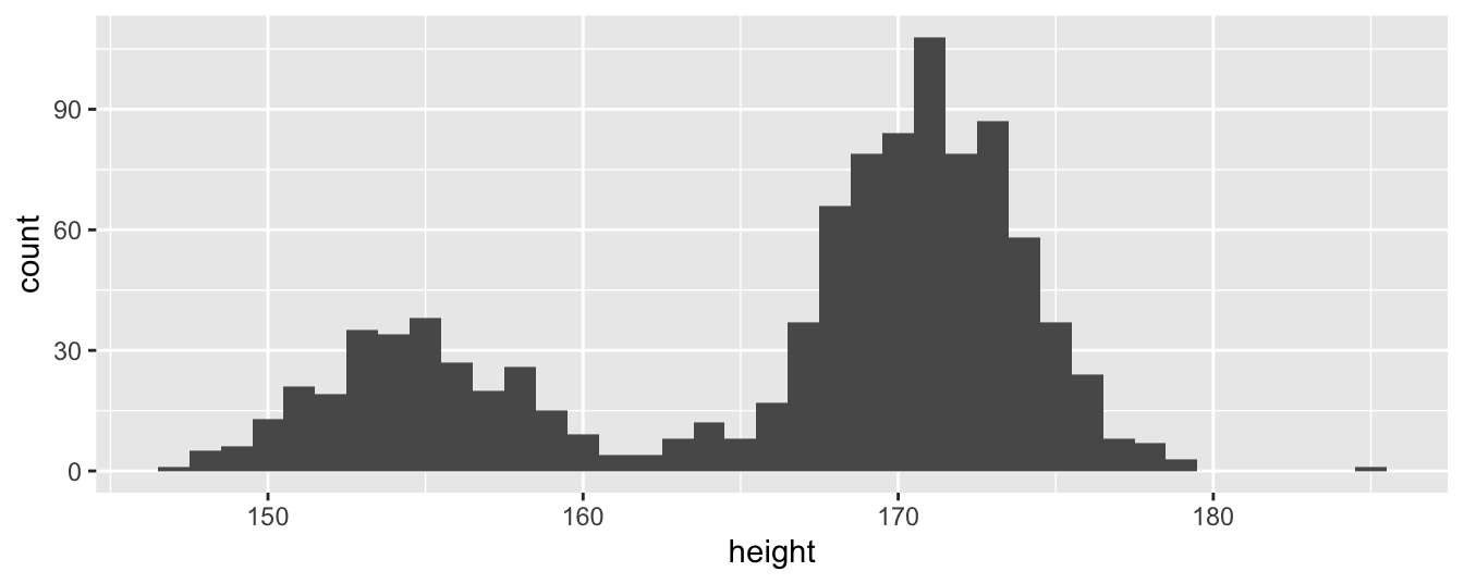
Now we make a function to draw multiple (n_samples) samples (each of sample_size size) from the distribution supplied as the dgf argument and calculate the mean for each sample.
Here we draw 10,000 samples of 1000 from bimodal_dgf(). (You may be pleasantly surprised to learn that we can just pass one R function—bimodal_dgf()—into another!)
set.seed(2023)
bimodal_sample_stats <- get_means(sample_size = 1000,
                                  n_samples = 10000,
                                  dgf = bimodal_dgf)
Now we make a small function make_clt_plot() to plot the histogram for the variable mean in the supplied data frame df, along with the normal distribution matching the mean and standard deviation of mean.
make_clt_plot <- function(df) {
  df |>
    ggplot(aes(x = mean)) +
    geom_histogram(aes(y = after_stat(density)), fill = "green",
                   binwidth = sd(df$mean) / 10) +
    geom_vline(aes(xintercept = mean(mean), color = "red")) +
    stat_function(fun = dnorm,
                  args = list(mean = mean(df$mean),
                              sd = sd(df$mean)),
                  color = "blue") +
    theme(legend.position = "none")
}
Using this function with bimodal_sample_stats, we see in Figure 5.2 that, while the underlying distribution is bimodal, the distribution of means is very close to normal.
make_clt_plot(bimodal_sample_stats)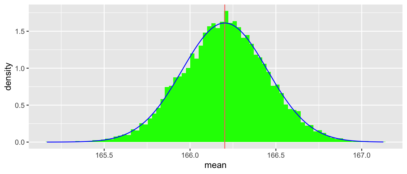
We can combine the get_means() and make_clt_plot() functions into a single function clt_demo() that allows us to make a plot of the distribution of means with an overlaid normal distribution so that we can see how well the latter approximates the former for a given sample size (sample_size) and DGF (dgf).
clt_demo <- function(sample_size, n_samples, dgf) {
  get_means(sample_size, n_samples, dgf) |>
    make_clt_plot()
}
We use clt_demo() for Figure 5.3, which is like Figure 5.2, but for sample_size = 100.
clt_demo(sample_size = 100, n_samples = 10000, bimodal_dgf)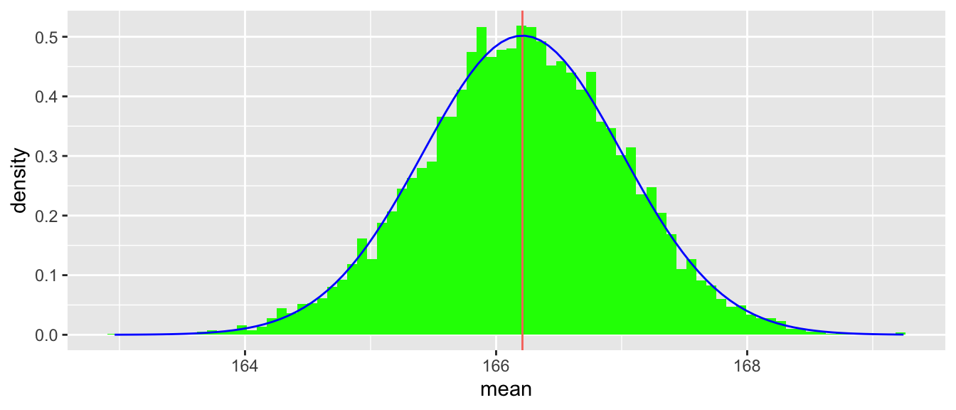
5.3.4 Unknown distribution: Bootstrapping
Above we considered the possibility that we had a normally distributed variable, but didn’t know the standard deviation. We saw that we can easily use the sample we have to estimate that standard deviation. In fact, we can go further and use the sample to generate information about arbitrary features of the distribution of the underlying variable.
The bootstrapping approach in this setting proceeds as follows:
- Take a with-replacement sample of size \(n\) from our sample.
- Calculate the mean for that sample.
- Repeat steps 1 and 2 many times.
- Use the distribution from step 3 to calculate estimates of relevant parameters (e.g., the standard deviation).
We can use the sample we created above (bimodal_sample) for this purpose. Here we calculate 10,000 samples. We first construct the get_bs_mean() function to perform steps 1 and 2.
We use then map_vec() to perform step 3.
We might simply use the results of our bootstrapping procedure to estimate the standard error of our mean estimates.
se_est <- sd(bs_stats$mean)
se_est
[1] 0.2489343But we could also use these results to evaluate the appropriateness of the normal approximation. Figure 5.4 suggests that the approximation is quite good in this case.
make_clt_plot(bs_stats) 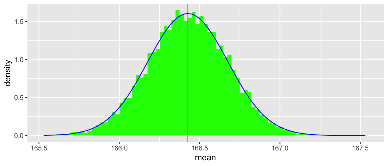
Here we have barely scratched the surface of what can be done with bootstrapping analysis. In some settings, we can use bootstrapping to read off critical values without needing to rely on the distribution approximating a normal distribution. We will see bootstrapping approaches again below and we discuss them in more detail in subsequent chapters.
5.3.5 Exercises
What is the relation between critical values and p-values using z-statistics and t-statistics? (Hint: Use R functions such as
qt(p/2, df = sample_size - 1)andqnorm(0.025)for various significant levels and sample sizes.)Explain how the output of the following code relates to the statistical tests above. Why does this relationship exist?
Examine
clt_demo(sample_size, n_samples = 10000, bimodal_dgf)for different values ofsample_size. At what value ofsample_sizedoes the underlying non-normality ofbimodal_dgf()become apparent?Using the value for
sample_sizeyou calculated in the previous question, what effect does varyingn_sampleshave on the distribution? How do you interpret the pattern here?Create your own data-generating function (say,
my_dgf()) likebimodal_dgf(). This function should embody the distribution of a random variable and it should have a single required argumentnfor the size of the sample that it returns. Examine the output ofclt_demo()for your function. (Hint: Likebimodal_dgf(), you might find it helpful to use R’s built-in functions, such assample()andrnorm()to make your function.)
5.4 Differences in means
As we saw in Chapter 3, we are often interested in the differences in means between two groups of observations. Suppose that the first group has \(n_0\) observations and is drawn from a distribution with mean of \(\overline{x}_0\) and standard deviation \(\sigma_0\), and the second group has \(n_1\) observations and is drawn from a distribution with mean of \(\overline{x}_1\) and standard deviation \(\sigma_1\).
Given the maintained assumption of independence of the observations here, the two sample means are independently distributed. The difference between the means of the two groups \(\overline{x}_1 - \overline{x}_0\) has variance equal to the sum of the variances of each mean.
\[ \mathrm{var}(\overline{x}_1 - \overline{x}_0) = \frac{\sigma^2_1}{n_1} + \frac{\sigma^2_0}{n_0} \] Taking the square root of this gives the standard error of the difference in means.
\[ \mathrm{se}(\overline{x}_1 - \overline{x}_0) = \sqrt{\frac{\sigma^2_1}{n_1} + \frac{\sigma^2_0}{n_0}} \] Again, with large-enough samples, we can often assume that the difference in means will be approximately normally distributed.
One important point to note is that if the null hypothesis is \(\mu_0 = \mu_1 = 0\), then it may be tempting to think that if the null hypothesis \(\mu_1 \leq 0\) is rejected (in favour of \(H_1: \mu_1 > 0\)) while the null hypothesis \(\mu_0 \leq 0\) is not, then we can conclude that the null hypothesis \(\mu_1 \leq \mu_0\) can thereby be rejected (in favour of \(H_1: \mu_1 > \mu_0\)). This reasoning is erroneous, as we will demonstrate.
Imagine that our sampling procedure will draw 1,000 observations from each of two groups and that we will compare the means of these two sub-samples. We will construct 10,000 such samples; we do this by constructing them in turn using the get_means() function from above with dgf = rnorm.
set.seed(2023)
sample_0_stats <- get_means(sample_size = 1000,
                            n_samples = 10000,
                            dgf = rnorm)

sample_1_stats <- get_means(sample_size = 1000,
                            n_samples = 10000,
                            dgf = rnorm)
We then merge these two samples by the sample identifier (i) and for each sample, we calculate the difference in means and the standard error of the difference using the formula above. From these values, we can calculate the z-statistic for each difference.
merged_stats <-
  sample_0_stats |>
  inner_join(sample_1_stats, by = "i", suffix = c("_0", "_1")) |>
  mutate(mean_diff = mean_1 - mean_0,
         se_diff = sqrt(se_0^2 + se_1^2),
         z_diff = mean_diff / se_diff)
Let’s assume that the size of our test is \(\alpha = 0.05\). Because we are using two-tailed tests, we set the critical value to the absolute value of \(\Phi^{-1}(\alpha/2).\)
The correct way to evaluate difference in means is to consider the difference significant if (1) \(\left|z_{\text{diff}}\right| > c\). However, some researchers will consider the difference significant if either (2) \(|z_1| > c\) while \(|z_0| \leq c\) or (3) \(|z_0| > c\) while \(|z_1| \leq c\). And there is a risk that researchers will take the opportunity to declare the difference “statistically significant” if any of the conditions (1), (2), or (3) is met.
Below we calculate the proportion of samples for which the null hypothesis is rejected based on condition (1) (prop_sig_diff), based on conditions (2) or (3) (prop_sig_diff_alt), or based on conditions (1), (2), or (3) (prop_sig_diff_choice).
merged_stats |>
  mutate(sig_diff = abs(z_diff) > crit_value,
         sig_1 = abs(z_1) > crit_value,
         sig_0 = abs(z_0) > crit_value) |>
  summarize(prop_sig_diff = mean(sig_diff),
            prop_sig_diff_alt = mean((sig_1 & !sig_0) | (sig_0 & !sig_1)),
            prop_sig_diff_choice = mean(sig_diff | (sig_1 & !sig_0) |
(sig_0 & !sig_1)))| prop_sig_diff | prop_sig_diff_alt | prop_sig_diff_choice |
|---|---|---|
| 0.0508 | 0.0967 | 0.1161 |
5.4.1 Discussion question
What is the issue implied by the statistics reported in Table 5.1? What is the correct approach implied by these statistics? Why might researchers prefer to have a choice regarding the test to be used?
5.5 Inference with regression
In practice, most statistical inference in accounting research relates to the hypotheses about regression coefficients. Fortunately, most of the concepts we have seen above with inference about means carry over to inference in regression settings.
When the OLS estimator is unbiased, the expected value of \(\hat{\beta}\) will be \(\beta\), but \(\hat{\beta}\) is just an estimate and will typically differ from the true value, as we can see by substituting the value of \(y\) into the equation for \(\hat{\beta}\) and doing some algebra. Note that below we use the facts that \(\mathbb{E} \left[\hat{\beta} - \beta \right]\) is zero (implied by the expression below) and that the variance of a zero-mean vector \(Z\) equals \(\mathbb{E} \left[ZZ' \right]\).
\[ \begin{aligned} \hat{\beta} &= (X^{\mathsf{T}}X)^{-1}X^{\mathsf{T}}y \\ &= (X^{\mathsf{T}}X)^{-1}X^{\mathsf{T}}(X\beta + \epsilon) \\ &= (X^{\mathsf{T}}X)^{-1}X^{\mathsf{T}}X\beta + (X^{\mathsf{T}}X)^{-1}\epsilon \\ & = \beta + (X^{\mathsf{T}}X)^{-1}X^{\mathsf{T}}\epsilon \\ \hat{\beta} - \beta &= (X^{\mathsf{T}}X)^{-1}X^{\mathsf{T}}\epsilon \\ \mathrm{var} (\hat{\beta}|X) &= \mathbb{E} \left[(X^{\mathsf{T}}X)^{-1}X^{\mathsf{T}} \epsilon \epsilon' X (X^{\mathsf{T}}X)^{-1} | X\right] \\ &= (X^{\mathsf{T}}X)^{-1}X^{\mathsf{T}} \mathbb{E} \left[\epsilon \epsilon' | X\right] X (X^{\mathsf{T}}X)^{-1} \end{aligned} \]
Now if \(\mathbb{E} \left[\epsilon_i \epsilon_j \right] = 0, \forall i \neq j\), then \(\mathbb{E} \left[\epsilon \epsilon' | X\right]\) will be a diagonal matrix with each element on the main diagonal equal to \(\sigma^2_i\), the variance of \(\epsilon\) for observation \(i\) (i.e., \(\mathrm{var} (\epsilon_i)\)). And if \(\mathbb{E} [\sigma^2_i |X ] = \sigma^2\) for all \(i\), then we have:
\[ \begin{aligned} \Sigma &:= \mathrm{var} (\hat{\beta}|X) \\ &= \sigma^2 (X^{\mathsf{T}}X)^{-1}X^{\mathsf{T}}X (X^{\mathsf{T}}X)^{-1} \\ &= \sigma^2 (X^{\mathsf{T}}X)^{-1} \\ \end{aligned} \]
This is the familiar result under the “standard” OLS assumptions, including the assumption that \(\mathbb{E} [\sigma^2_i |X ] = \sigma^2\) for all \(i\), which is known as homoskedasticity.
One issue is that we do not observe \(\sigma^2\), but we can estimate it using the standard formula
\[ \hat{\sigma}^2 = \frac{1}{N-k} \sum_{i=1}^N \hat{\epsilon}_i^2 \] where \(\hat{\epsilon}_i\) is the regression residual for observation \(i\) and \(N - k\) incorporates a degrees-of-freedom correction. (Note that \(k = 2\) when we have one regressor in addition to a constant term.) Putting the above together, we have
\[ \hat{\Sigma} = \hat{\sigma}^2 (X^{\mathsf{T}}X)^{-1} \]
This is also the standard approach to estimating the variance of coefficients in statistical software, including the lm() function in R. To confirm this, let’s create a test data set, calculate regression statistics “by hand” and then compare results with those provided by the lm() function.
To make this more concrete, let’s consider some simulated data. Specifically, we generate 1000 observations with \(\beta = 1\) and \(\sigma = 0.2\).
We next construct \(X\) as a matrix comprising a column of ones (to estimate the constant term) and a column containing \(x\).
We then calculate \(\beta\) and residuals by hand.
We can now calculate \(\hat{\sigma}^2\) and then \(\hat{\Sigma}\). This allows us to calculate the estimated standard errors of the estimated coefficients as the square root of the diagonal elements of \(\hat{\Sigma}\) and then the t-statistics for each coefficient by dividing each element of \(\hat{\beta}\) by its estimated standard error. Results from the following code are shown in Table 5.2.
| b | se | t | p |
|---|---|---|---|
| 0.007540 | 0.006440 | 1.171 | 0.242 |
| 0.997647 | 0.006321 | 157.829 | 0.000 |
Now, let’s compare the results seen in Table 5.2 with those in Table 5.3, which are obtained from the following code, which applies summary() to a model estimated using lm().
fm <- lm(y ~ x)
coefficients(summary(fm))lm()
| Estimate | Std. Error | t value | Pr(>|t|) | |
|---|---|---|---|---|
| (Intercept) | 0.007540 | 0.006440 | 1.171 | 0.242 |
| x | 0.997647 | 0.006321 | 157.829 | 0.000 |
You may have noticed that these approaches to testing hypotheses about regression coefficients are analogous to those used to test hypotheses about means in Sections 5.3.1 and 5.3.2. Similarly, we might use asymptotic methods or bootstrapping to test hypotheses about regression coefficients. In fact, the assumptions required to yield regression coefficients that follow the \(t\) distribution—such as normally distributed error terms—are generally implausible in most research settings and in practice most inferences are justified based on asymptotic results and assumptions of approximately normal distributions in the finite samples of actual research. In fact, all the approaches discussed in Section 5.6 are justified asymptotically.
In the remainder of this section, we discuss how bootstrapping can be applied to regression analysis. The bootstrapping approach in this setting proceeds as follows:
- Take a with-replacement sample of size \(n\) from our sample of data.
- Calculate the regression coefficients for that sample.
- Repeat steps 1 and 2 many times.
- Use the distribution above to calculate estimates of relevant parameters (e.g., the standard error of regression coefficients).
To demonstrate this, we put our y and x variables above into a data frame.
df <- tibble(y, x)We create a function (get_bs_coefs()) that performs steps 1 and 2.
We then use map() to repeat these steps 10,000 times.
set.seed(2021)
bs_coefs <-
  tibble(i = 1:n_samples) |>
  mutate(coefs = map(i, \(x) get_bs_coefs(data = df))) |>
  unnest_wider(coefs)
We can then calculate the standard deviation of the estimated regression coefficients as an estimate of their standard errors. Here we use across() to summarize multiple columns in one step and display results in Table 5.4.9
bs_coefs |>
  select(-i) |>
summarize(across(everything(), sd))| (Intercept) | x |
|---|---|
| 0.0064542 | 0.0064964 |
5.6 Dependence
In generating data in Chapter 3, we assumed that the errors and regressors were independent. However, most of the empirical accounting research uses panel data sets, typically repeated observations on a set of firms over time. In these settings, it is reasonable to assume that regressors (\(X\)) and errors (\(\epsilon\)) are correlated both across firms (i.e., cross-sectional dependence) and over time (i.e., time-series dependence).
While White (1980) standard errors are consistent in the presence of heteroskedasticity, it is well known that both OLS and White produce misspecified test statistics when either form of dependence is present.
Gow et al. (2010) demonstrate that accounting researchers use a variety of approaches to address the issues of cross-sectional and time-series dependence widely understood to be present in common research settings. The literature survey in Gow et al. (2010) identified a number of common approaches: Fama-MacBeth, Newey-West, the “Z2” statistic, and standard errors clustered by firm, industry, or time.
5.6.1 Newey-West
The White (1980) approach was generalized by Newey and West (1987) to give a covariance matrix estimator robust to both heteroskedasticity and serial correlation. While the Newey-West procedure was developed in the context of a single time series, Gow et al. (2010) show it is frequently applied in panel data settings, where its use is predicated on cross-sectional independence. Assessing the performance of Newey-West in the presence of both cross-sectional and time-series dependence, Gow et al. (2010) find that it produces misspecified test statistics with even modest levels of cross-sectional dependence.
5.6.2 Fama-MacBeth
The Fama-MacBeth approach (Fama and MacBeth, 1973) addresses concerns about cross-sectional correlation. The original Fama-MacBeth approach—which Gow et al. (2010) label “FM‑t”—involves estimating T cross-sectional regressions (one for each period) and basing inferences on a t-statistic calculated as
\[ t = \frac{\overline{\beta}}{\mathit{se}(\hat{\beta})}\text{, where } \overline{\beta} = \frac{1}{T} \sum_{t=1}^T \hat{\beta}_t\]
and \(\mathit{se}(\hat{\beta})\) is the standard error of the coefficients based on their empirical distribution. When there is no cross-regression (i.e., time-series) dependence, this approach yields consistent estimates of the standard error of the coefficients as T goes to infinity. However, cross-regression dependence in errors and regressors causes Fama-MacBeth standard errors to be understated (Cochrane, 2009; Schipper and Thompson, 1983).
To illustrate the Fama-MacBeth approach, we will generate a data set using the simulation approach of Gow et al. (2010), which is available using the get_got_data() function found in the farr package. The parameters Xvol and Evol relate to the cross-sectional dependence of \(X\) and \(\epsilon\), respectively. The parameters rho_X and rho_E relate to the time-series dependence of \(X\) and \(\epsilon\), respectively. We get 10 years of simulated data on 500 firms and store the data in the data frame named test.
set.seed(2021)
test <- get_got_data(N = 500, T = 10,
                     Xvol = 0.75, Evol = 0.75,
                     rho_X = 0.5, rho_E = 0.5)
We first estimate using nest() from tidyr to organize the relevant data by year. We then use the map() function from the purrr package twice. We first use map() to estimate the regression by year and put the fitted models in a column named fm. We then use map() again to extract the coefficients from the fm column and put them in the coefs column.10
We then use the unnest_wider() function from the tidyr package to extract the data in coefs into separate columns in the data frame coefs_df.
coefs_df <-
  results |>
  unnest_wider(coefs) |>
  select(year, `(Intercept)`, x)
The data frame coefs_df contains the results of the first step of the Fama-MacBeth approach, which are shown in Table 5.5.
coefs_df| year | (Intercept) | x |
|---|---|---|
| 1 | 1.6356 | 0.9514 |
| 2 | 2.7017 | 0.9899 |
| 3 | -1.1093 | 0.9078 |
| 4 | -0.3491 | 1.0952 |
| 5 | -0.8629 | 1.0035 |
| 6 | -0.4451 | 0.9104 |
| 7 | -0.2011 | 1.0507 |
| 8 | 1.5738 | 0.8011 |
| 9 | -2.7727 | 0.9517 |
| 10 | 0.8072 | 0.9843 |
The second step of the Fama-MacBeth approach involves calculating the mean and standard error of the estimated coefficients. As we see in the exercises, regression of the time-series of coefficients on a constant produces the required mean and standard error.
Two common variants of the Fama-MacBeth approach appear in the accounting literature. The first variant, which Gow et al. (2010) label “FM‑i”, involves estimating firm- or portfolio-specific time-series regressions with inferences based on the cross-sectional distribution of coefficients. FM-i had been used extensively in the accounting literature prior to Gow et al. (2010).
FM-i is appropriate if there is time-series dependence but not cross-sectional dependence. However, it is difficult to identify such circumstances in real research settings and we do not discuss FM-i further.11
The second common variant of the FM‑t approach, which Gow et al. (2010) label FM‑NW, is intended to correct for serial correlation in addition to cross-sectional correlation. FM‑NW modifies FM‑t by applying a Newey-West adjustment in an attempt to correct for serial correlation. While a number of studies claimed that FM‑NW produces a conservative estimate of statistical significance, they did so without any formal evaluation of FM‑NW.
Implementing FM-NW is straightforward using the sandwich package. In get_nw_vcov(), we simply apply NeweyWest() from the sandwich package to the fitted FM-t model to recover the FM-NW covariance matrix.12
get_nw_vcov <- function(fm, lag = 1) {
  NeweyWest(fm, lag = lag, prewhite = FALSE, adjust = TRUE)
}
In Table 5.6, we tabulate the Fama-MacBeth coefficients twice: once with the default standard errors and once with Newey-West standard errors.
modelsummary(dvnames(c(fms, fms)),
             coef_rename = c('(Intercept)' = 'Estimate'),
             vcov = c(map(fms, vcov),
                      map(fms, get_nw_vcov)),
             estimate = "{estimate}{stars}",
             output = "kableExtra",
             coef_omit = "^factor",
             gof_map = c("nobs", "r.squared"),
             stars = c('*' = .1, '**' = 0.05, '***' = .01)) |>
add_header_above(c(" " = 1, "FM-t" = 2, "FM-NW" = 2))| (Intercept) | x | (Intercept) | x | |
|---|---|---|---|---|
| Estimate | 0.098 | 0.965*** | 0.098 | 0.965*** |
| (0.506) | (0.026) | (0.457) | (0.020) | |
| Num.Obs. | 10 | 10 | 10 | 10 |
| R2 | 0.000 | 0.000 | 0.000 | 0.000 |
Gow et al. (2010) show that FM-NW fails to address serial correlation and offer two explanations for this failure. “First, FM‑NW generally involves applying Newey-West to a limited number of observations, a setting in which Newey-West is known to perform poorly. Second, FM‑NW applies Newey-West to a time-series of coefficients, whereas the dependence is in the underlying data” (Gow et al., 2010, p. 488). For example, without the underlying data, it is not possible to discern whether the sequence {2.1, 1.8, 1.9, 2.2, 2.3} represents highly auto-correlated draws from a mean-zero distribution or independent draws from a distribution with mean 2. As such, we do not examine FM-NW any further.
To estimate FM-t, we can use the pmg() function from the plm package. We simply specify the variable containing the relevant index (i.e., the \(t\) in FM-t).
fm_fmt <- pmg(y ~ x, data = test, index = "year")Because pmg objects created using the plm package do not support the modelsummary() function out of the box, we implement tidy() and glance() functions so that modelsummary() knows how to handle these.13
tidy.pmg <- function(x, ...) {
    res <- summary(x)
    tibble(
      term      = names(res$coefficients),
      estimate  = res$coefficients,
      std.error = se(res),
      statistic = res$coefficients / se(res),
      p.value   = pvalue(res))
}

glance.pmg  <- function(x, ...) {
    res <- summary(x)
    tibble(
      r.squared     = res$rsqr,
      adj.r.squared = res$r.squared,
      nobs          = length(res[[2]]))
}
In Table 5.7, we can see that the results using pmg() line up with those we calculated “by hand” above.
modelsummary(fm_fmt,
             estimate = "{estimate}{stars}",
             coef_omit = "^factor",
             gof_map = c("nobs", "r.squared"),
stars = c('*' = .1, '**' = 0.05, '***' = .01))pmg()
| (1) | |
|---|---|
| (Intercept) | 0.098 |
| (0.506) | |
| x | 0.965*** |
| (0.026) | |
| Num.Obs. | 5000 |
| R2 | 0.786 |
5.6.3 Z2 statistic
According to Gow et al. (2010, p. 488), the Z2 statistic first appeared in 1994 and was used in a number of subsequent studies in accounting research. The Z2‑t statistic is calculated from the t-statistics from separate period-specific cross-sectional regressions as:
\[ \textit{Z2} = \frac{\overline{t}}{\mathit{se}(\hat{t})}\text{, where } \overline{t} = \frac{1}{T} \sum_{t=1}^T \hat{t}_t\]
\(\mathit{se}(\hat{t})\) is the standard error of the t-statistics based on their empirical distribution, and T is the number of time periods in the sample.14 Several studies claimed that Z2 adjusts for cross-sectional and serial correlation, but offered no basis for this claim. Gow et al. (2010) found no prior formal analysis of the properties of the Z2 statistic and found that Z2 suffers from cross-regression dependence in the same way as the Fama-MacBeth approach does.
5.6.4 One-way cluster-robust standard errors
A number of studies in the survey by Gow et al. (2010) use cluster-robust standard errors, with clustering either along a cross-sectional dimension (e.g., analyst, firm, industry, or country) or along a time-series dimension (e.g., year). Gow et al. (2010) refer to the former as CL‑i and the latter as CL‑t. Cluster-robust standard errors (also referred to as Huber-White or Rogers standard errors) were proposed by White (1984) as a generalization of the heteroskedasticity-robust standard errors of White (1980). With observations grouped into \(G\) clusters of \(N_g\) observations, for \(g\) in \({1, \dots, G}\), the covariance matrix is estimated using the following expression:
\[ \hat{V}(\hat{\beta}) = (X'X)^{-1} \hat{B} (X'X)^{-1} \text{, where } \hat{B} = \sum_{g=1}^G X'_g u_g u'_g X_g \tag{5.1}\] where \(X_g\) is the \(N_g \times K\) matrix of regressors, and \(u_g\) is the \(N_g\)-vector of residuals for cluster \(g\). If each cluster contains a single observation, Equation 5.1 yields the White (1980) heteroskedasticity-consistent estimator.
While one-way cluster-robust standard errors permit correlation of unknown form within each cluster, they assume on a lack of dependence across clusters. Gow et al. (2010) demonstrate that t-statistics for CL‑t are overstated in the presence of time-series dependence and t-statistics for CL‑i are overstated in the presence of cross-sectional dependence. So when both forms of dependence are present, CL‑t and CL‑i will both produce inflated t-statistics.
Because cluster-robust methods assume independence across clusters, clustering by, say, industry-year does not produce standard errors robust to either within-industry or within-year dependence. In fact, this requires that there be neither time-series nor cross-industry dependence (i.e., no dependence between observations for industry \(j\) in year \(t\) and those in industry \(j\) in year \(t+1\) or those in industry \(k\) in year \(t\)). More concretely, clustering by firm-year when the observations are firm-years simply produces White standard errors.
5.6.5 Two-way cluster-robust standard errors
Thompson (2011) and Cameron et al. (2011) developed an extension of cluster-robust standard errors that allows for clustering along more than one dimension.
In contrast to one-way clustering, two-way clustering (CL‑2) allows for both time-series and cross-sectional dependence. For example, two-way clustering by firm and year allows for within-firm (time-series) dependence and within-year (cross-sectional) dependence (e.g., the observation for firm \(j\) in year \(t\) can be correlated with that for firm \(j\) in year \(t+1\) and that for firm \(k\) in year \(t\)). To estimate two-way cluster-robust standard errors, the expression in Equation 5.1 is evaluated using clusters along each dimension (for example, clustered by industry and clustered by year) to produce estimated covariance matrices \(V_1\) and \(V_2\). The same expression is calculated for the “intersection” clusters (in our example, observations within an industry-year) to yield the estimated covariance matrix \(V_I\). The estimated two-way cluster-robust covariance matrix \(V\) is then calculated as \(V = V_1 + V_2 - V_I\). Packages available for R make it straightforward to implement two-way cluster-robust standard errors and we demonstrate their use below.
5.6.6 Calculating standard errors
In the following code, we use functions from three libraries (sandwich, plm, and fixest) to estimate seven models. The fixest library provides the feols() function as an extension to lm() that allows for fixed effects, instrumental variables, and clustered standard errors. We demonstrated basic usage of feols() in Chapter 3. We will discuss the use of feols() with fixed effects and instrumental variables in later chapters. Here we just use feols() to get clustered standard errors.
fms <- list(OLS = lm(y ~ x, data = test),
            White = lm(y ~ x, data = test),
            NW = plm(y ~ x, test, index = c("firm", "year"),
                     model = "pooling"),
            `FM-t` = pmg(y ~ x, test, index = "year"),
            `CL-i` = feols(y ~ x, vcov = ~ firm, data = test),
            `CL-t` = feols(y ~ x, vcov = ~ year, data = test),
            `CL-2` = feols(y ~ x, vcov = ~ year + firm, data = test))
Note that the coefficient estimates will be equal for every model except the FM-t model.15 The only difference between the six models other than FM-t will be the estimated standard errors.
For most of the models, we can produce the covariance matrix using vcov(). However, for White, we need to replace the default covariance matrix (so far there is no difference between OLS and White) with the result of calling vcovHC() from the sandwich package with type = "HC1".16 For NW, we call vcovNW() from the plm package.
Table 5.8 provides estimates and standard errors calculated using a number of approaches.
modelsummary(fms,
             vcov = vcovs,
             estimate = "{estimate}{stars}",
             coef_omit = "^factor",
             gof_map = c("nobs", "r.squared"),
stars = c('*' = .1, '**' = 0.05, '***' = .01))| OLS | White | NW | FM-t | CL-i | CL-t | CL-2 | |
|---|---|---|---|---|---|---|---|
| (Intercept) | 0.021 | 0.021 | 0.021 | 0.098 | 0.021 | 0.021 | 0.021 |
| (0.026) | (0.026) | (0.027) | (0.506) | (0.023) | (0.492) | (0.492) | |
| x | 1.266*** | 1.266*** | 1.266*** | 0.965*** | 1.266*** | 1.266*** | 1.266*** |
| (0.027) | (0.021) | (0.021) | (0.026) | (0.018) | (0.172) | (0.172) | |
| Num.Obs. | 5000 | 5000 | 5000 | 5000 | 5000 | 5000 | 5000 |
| R2 | 0.305 | 0.305 | 0.305 | 0.786 | 0.305 | 0.305 | 0.305 |
With the exception of OLS, all methods depicted in Table 5.8 have asymptotic foundations and can have problems in small-sample settings. For example, FM‑t is predicated on \(T \to \infty\) and its distribution may not be well approximated by the normal distribution when \(T = 10\). Cameron et al. (2008) document that cluster-robust methods will over-reject a true null when the number of clusters is small, an issue that can be attributed to the use of limiting distributions in making inferences in small samples (e.g., using the standard 1.64, 1.96, and 2.58 critical values from the normal distribution).
Accordingly, researchers should exercise caution when applying any asymptotic methods (e.g., FM-t, CL-t, or CL-2) when the number of time periods is small. Nonetheless, Gow et al. (2010) find CL‑2 produces unequivocally better inferences in the presence of time-series and cross-sectional dependence than any of the other methods considered in Table 5.8 even with as few as 10 clusters. Additionally, as there are approaches to address this concern (e.g., Cameron et al., 2008 identify corrections based on bootstrapping methods), Gow et al. (2010) argue that having few clusters does not justify relying on approaches that are not robust to cross-sectional and time-series dependence.
5.6.7 Exercises
Verify either by direct computation using the data in
coefs_dfor using a little algebra that regressing the first-stage coefficients on a constant (as we did above) yields the desired second-stage results for FM-t.Assume that the null hypothesis is \(H_0: \beta = 1\). Using the reported coefficients and standard errors for each of the methods listed in Table 5.8 (i.e., OLS, White, NW, FM-t, CL-i, CL-t, CL-2), for which methods is the null hypothesis rejected?
Based on the analysis in Gow et al. (2010), when should you use the FM-NW or Z2 approaches? What factors might have led researchers to use these approaches and make unsubstantiated claims about them (e.g., robustness to cross-sectional and time-series dependence)?
If FM-i is, as Gow et al. (2010) show, so inappropriate for the situations in which it was used, why do you think it was used in those situations?
Gow et al. (2010) refer to “the standard 1.64, 1.96, and 2.58 critical values.” Using the
pnorm()function, determine the p-value associated with each of these critical values. Are these one-tailed or two-tailed p-values? The values of 1.64, 1.96, and 2.58 are approximations. Which function in R allows you to recover the precise critical values associated with a chosen p-value? (Hint: Read the help provided by? pnormin R.) Provide the critical values to four decimal places.
5.7 Further reading
Chapter 26 of R for Data Science covers the topic of iteration, including the functions across() and map() discussed above. That chapter also discusses anonymous functions and the unnest_wider() function.
The discussion above is a very selective introduction to statistical inference and there are a number of basic topics we have not addressed. Chapter 3 of Davidson and MacKinnon (2004) discusses the covariance matrix of OLS estimates along with other statistical properties of OLS. Angrist and Pischke (2008) provide an excellent treatment of issues related to standard errors.
We provided a very intuitive introduction to ideas related to laws of large numbers and central limit theorems. Chapter 4 of Davidson and MacKinnon (2004) provides a more thorough and rigorous introduction to these topics.
We did not discuss joint hypotheses (i.e., those involving more than one coefficient) or hypotheses that impose non-linear restrictions. Chapter 4 of Kennedy (2008) provides an intuitive introduction to these topics.
We examine some of these issues in Chapter 19.↩︎
Referring to these results in the plural (“laws” and “theorems”) without the definite article (“the”) and in lower case is intended to indicate that these results are actually sets of closely related results exhibiting the general pattern that stronger assumptions (imposed on the random variables in question) lead to “stronger” results.↩︎
If speaking to a careful econometrician, one should be careful about conflating consistency and unbiasedness, as there exist estimators that are always biased in finite samples, but are consistent and estimators that are unbiased, but not consistent.↩︎
We eschew the word “random” here lest it be misinterpreted in an implausible “equal probability of existing” sense.↩︎
Type
? set.seedin R to learn more.↩︎There are base R equivalents to the functions provided by
purrr, such asMap()andlapply(). Perhaps the main benefit of using thepurrrfunctions is that they are easier to learn because there is greater consistency across functions.↩︎We also ignore the various semantic debates, such as whether one “accepts” alternative hypotheses and “rejects” null hypotheses or whether other words better describe what is going on.↩︎
This is because of the symmetry of the standard normal distribution around zero.↩︎
The
across()function is covered in some detail in Chapter 26 of R for Data Science.↩︎Note that we use the shortcut form that allows us to write
function(df) lm(y ~ x, data = df)as simply\(df) ~ lm(y ~ x, data = df).↩︎In fact, Gow et al. (2010) found that FM‑i was most frequently used when cross-sectional dependence was the primary issue, such as when returns are the dependent variable.↩︎
The options here are chosen to line up with the
NeweyWestPanelStata()function provided by Gow et al. (2010) at https://go.unimelb.edu.au/dzw8. This function in turn was verified to line up with thenewey.adofunction from Stata.↩︎See the “extension and customization” page of the
modelsummarydocumentation for details: https://go.unimelb.edu.au/vzw8.↩︎As discussed in Gow et al. (2010), just as there are FM-i and FM-t statistics, there were Z2-i and Z2-t statistics. We only discuss the Z2-t variant here.↩︎
The estimates from the
FM-tmodel can be viewed as invoking pooled OLS with a different weighting for observations by year.↩︎The default value is
type = "HC3", which is actually preferred for many purposes. We useHC1to line up with the approaches discussed in Gow et al. (2010) and defer discussion of the differences betweenHC1,HC2, andHC3to Chapter 23.↩︎