22 Regression discontinuity designs
This is the published R edition of the book. A Python version of the book is available at era_pl_book.
Over the last twenty years or so, the regression discontinuity design (RDD) has seen a dramatic rise in popularity among researchers. Cunningham (2021) documents a rapid increase in the number of papers using RDD after 1999 and attributes its popularity to its ability to deliver causal inferences with “identifying assumptions that are viewed by many as easier to accept and evaluate” than those of other methods. Lee and Lemieux (2010, p. 282) point out that RDD requires “seemingly mild assumptions compared to those needed for other non-experimental approaches … and that causal inferences from RDD are potentially more credible than those from typical ‘natural experiment’ strategies.”
Another attractive aspect of RDD is the availability of quality pedagogical materials explaining its use. The paper by Lee and Lemieux (2010) is a good reference, as are chapters in Cunningham (2021) and Angrist and Pischke (2008). Given the availability of these materials, we have written this chapter as a complementary resource, focusing more on practical issues and applications in accounting research. The goal of this chapter is to provide a gateway for you to either using RDD in your own research (should you find a setting with a discontinuity in a treatment of interest) or in reviewing papers using (or claiming to use) RDD.
A number of phenomena of interest to accounting researchers involve discontinuities. For example, whether an executive compensation plan is approved is a discontinuous function of shareholder support (e.g., Armstrong et al., 2013) and whether a debt covenant is violated is typically a discontinuous function of the realization of accounting ratios. So it is not surprising that RDD has attracted some interest of accounting researchers, albeit in a relatively small number of papers. Unfortunately, it is also not surprising that RDD has not always yielded credible causal inferences in accounting research, as we discuss below.
The code in this chapter uses the packages listed below. We load tidyverse because we use several packages from the Tidyverse. For instructions on how to set up your computer to use the code found in this book, see Section 1.2. Quarto templates for the exercises below are available on GitHub.
22.2 Fuzzy RDD
Fuzzy RDD applies when the cutoff \(x_0\) is associated not with a sharp change from “no treatment for any” to “treatment for all”, but with a sharp increase in the probability of treatment:
\[ P(D_i = 1 | x_i) = \begin{cases} g_1(x_i) & x_i \geq x_0 \\ g_0(x_i) & x_i < x_0 \end{cases}, \text{ where } g_1(x_0) > g_0(x_0) \] Note that sharp RDD can be viewed as a limiting case of fuzzy RDD in which \(g_1(x_i) = 1\) and \(g_0(x_i) = 0\).
The best way to understand fuzzy RDD is as instrumental variables meets sharp RDD. Suppose that shifting from just below to \(x_0\) to \(x_0\) or just above increases the probability of treatment by \(\pi\), then \(x_0\) is effectively random in that small range (thus addressing the first requirement for a valid instrument), it has an effect on treatment so long as \(\pi\) is sufficiently different from \(0\) (the second requirement) and its only effect on \(y\) over that small range occurs only through its effect on treatment (the third requirement).
The value for \(y_i\) just to the right of \(x_0\) will be approximately \(f(x_0) + D_i + \eta_i\) if treatment occurs and approximately \(f(x_0) + \eta_i\) if treatment does not occur. Given that treatment occurs with probability approximately equal to \(g_1(x_0)\) at or just to the right of \(x_0\), we have \(\mathbb{E}[y_{i} | x_0 \leq x_i < x_0 + \Delta] \approx f(x_0) + g_1(x_0) D_i + \eta_i\). The value for \(y_i\) just to the left of \(x_0\) will be approximately \(f(x_0) + D_i + \eta_i\) if treatment occurs and approximately \(f(x_0) + \eta_i\) if treatment does not occur. Given that treatment occurs with probability approximately equal to \(g_0(x_0)\) just to the left of \(x_0\), we have \(\mathbb{E}[y_{i} | x_0 - \Delta < x_i < x_0] \approx f(x_0) + g_0(x_0) D_i + \eta_i\). If \(g_1(x_0) - g_0(x_0) = \pi\), we have
\[ \begin{aligned} \lim_{\Delta \to 0} \left( \mathbb{E}[y_{i} | x_0 \leq x_i < x_0 + \Delta] - \mathbb{E}[y_{i} | x_0 - \Delta < x_i < x_0] \right) &= \mathbb{E}[y_{1i} | x_i = x_0] - \mathbb{E}[y_{0i} | x_i = x_0] \\ &= \mathbb{E}[y_{1i} - y_{0i} | x_i = x_0] \\ &= \pi \rho \end{aligned} \] We can estimate the effect of treatment, \(\rho\), by noting that
\[ \rho = \lim_{\Delta \to 0} \frac{\mathbb{E}[y_{i} | x_0 \leq x_i < x_0 + \Delta] - \mathbb{E}[y_{i} | x_0 - \Delta < x_i < x_0]}{\mathbb{E}[D_{i} | x_0 \leq x_i < x_0 + \Delta] - \mathbb{E}[D_{i} | x_0 - \Delta < x_i < x_0]} \]
Hoekstra (2009) is an excellent paper for building intuition with regard to fuzzy RDD and we recommend you read it. Figure 1 of Hoekstra (2009) demonstrates a sharp jump in the probability of enrolment (by \(0.388\)) at the flagship state university as students SAT score crosses the threshold for admission. Figure 2 of Hoekstra (2009) depicts an increase in future annual earnings (by \(0.095\)) as a student’s SAT score crosses the threshold for admission. This suggests that the estimated effect of enrolment on future earnings will be approximately \(0.095 \div 0.388 = 0.245\), which is actually quite close to the estimate of \(0.223\) in Table 1 of Hoekstra (2009).
22.3 Other issues
One issue with RDD is that the effect estimated is a local estimate (i.e., it relates to observations close to the discontinuity). This effect may be very different from the effect at points away from the discontinuity. For example, in designating a public float of $75 million as a threshold for applying the requirements of the Sarbanes-Oxley Act (SOX), the SEC may have reasoned that at that point the benefits of SOX were approximately equal to the costs of complying with it. If true, we would expect to see an estimate of approximately zero effect, even if there were substantial benefits of the law for shareholders of firms having a public float well above the threshold.
Another critical element of RDD is the bandwidth used in estimation (i.e., in effect how much weight is given to observations according to their distance from the cutoff). Gow et al. (2016) encourage researchers using RDD to employ methods that exist to estimate optimal bandwidths and the resulting estimates of effects (e.g., Imbens and Kalyanaraman, 2012). The rdrobust package used above provides various approaches to estimating optimal bandwidths and makes it easy to estimate RDD with alternative bandwidths. Credible results from RDD are likely to be robust to alternative bandwidth specifications.
Finally, one strength of RDD is that the estimated relation is often effectively univariate and easily plotted. As suggested by Lee and Lemieux (2010), it is highly desirable for researchers to plot both the underlying data and the fitted regression functions around the discontinuity. This plot will enable readers to evaluate the strength of the results. If there is a substantive impact associated with the treatment, this should be obvious from a plot of the actual data and the associated fitted function. Inspection of the plots in Hoekstra (2009) provides some assurance that the estimated effect is “there”. In contrast, the plots below using data from Bloomfield (2021) seem somewhat less compelling.
22.4 Sarbanes-Oxley Act
The Sarbanes-Oxley Act (SOX), passed by the US Congress in 2002 in the wake of scandals such as Enron and WorldCom, was arguably the most significant shift in financial reporting in recent history, with effects not only in the United States, but elsewhere in the world as measures taken in the United States were adopted in other jurisdictions. Iliev (2010, p. 1163) writes “the law’s main goal was to improve the quality of financial reporting and increase investor confidence.”
A key element of SOX is section 404 (SOX 404). Section 404(a) requires the Securities and Exchange Commission (SEC) to prescribe rules requiring management to include in annual reports “an assessment of … effectiveness of the internal control … for financial reporting.” Section 404(b) requires the company’s external auditor to “attest to, and report on, the assessment made by the management of the issuer.”
As discussed in Iliev (2010), SOX 404 generated significant controversy, with particular concerns being expressed about the costs of compliance, especially for smaller firms. In response to such concerns, the SEC required only companies whose public float exceeded $75 million in either 2002, 2003, or 2004 to comply with SOX 404 for fiscal years ending on or after 15 November 2004.4 Smaller companies were not required to submit management reports until fiscal 2007 and these did not require auditor attestation until 2010.
Iliev (2010) exploits the discontinuity in treatment around $75 million in public float and RDD to evaluate the effect of SOX 404 on audit fees and earnings management, finding evidence that SOX 404’s required management reports increased audit fees, but reduced earnings management.
Iliev (2010) “hand-collected” data on public float, and whether a firm was an accelerated filer, and whether it provided a management report under SOX 404 directly from firms’ 10-K filings.5
Some of these data are included in the iliev_2010 data frame included with the farr package.
iliev_2010# A tibble: 7,214 × 9
gvkey fyear fdate pfdate pfyear publicfloat mr af cik
<chr> <int> <date> <date> <dbl> <dbl> <lgl> <lgl> <dbl>
1 028712 2001 2001-12-31 2002-03-21 2002 21.5 FALSE FALSE 908598
2 028712 2002 2002-12-31 2002-06-28 2002 11.5 FALSE FALSE 908598
3 028712 2003 2003-12-31 2003-06-30 2003 13.9 FALSE FALSE 908598
4 028712 2004 2004-12-31 2004-06-30 2004 68.2 FALSE FALSE 908598
5 028712 2005 2005-12-31 2005-06-30 2005 26.4 FALSE FALSE 908598
6 013864 2001 2001-03-31 2001-07-06 2001 35.2 FALSE FALSE 819527
7 013864 2002 2002-03-31 2002-06-27 2002 31.8 FALSE FALSE 819527
8 013864 2003 2003-03-31 2002-09-30 2002 20.2 FALSE FALSE 819527
9 013864 2004 2004-03-31 2003-09-30 2003 18.3 FALSE FALSE 819527
10 013864 2005 2005-03-31 2004-09-30 2004 9.04 FALSE FALSE 819527
# ℹ 7,204 more rowsThe variables af and mf are indicators for a firm being an accelerated filer and for a firm filing a management report under SOX 404, respectively.
Iliev (2010, p. 1169) explains the criteria for a SOX 404 management report being required as follows:
All accelerated filers with a fiscal year ending on or after November 15, 2004 had to file a MR and an auditor’s attestation of the MR under Section 404. I denote these firms as MR firms. Companies that were not accelerated filers as of their fiscal year ending on or after November 15, 2004 did not have to file an MR in that year (non-MR firms). Those were companies that had a public float under $75 million in their reports for fiscal years 2002 (November 2002 to October 2003), 2003 (November 2003 to October 2004), and 2004 (November 2004 to October 2005).
The code producing the following data frame mr_req_df attempts to encode these requirements.
Interestingly, as seen in Table 22.1, there appear to be a number of firms that indicated that they were not accelerated filers and did not have to file a management report, despite appearing to meet the criteria.
| cik | fdate | pfdate | publicfloat |
|---|---|---|---|
| 1003472 | 2004-12-31 | 2005-03-09 | 141.9853 |
| 943861 | 2004-12-31 | 2005-03-24 | 168.5346 |
| 906780 | 2004-12-31 | 2005-03-01 | 171.6621 |
| 1085869 | 2004-12-31 | 2005-02-28 | 172.0916 |
| 29834 | 2004-12-31 | 2005-03-16 | 184.9020 |
| 1028205 | 2005-06-30 | 2005-08-15 | 279.1016 |
Using the firm with a CIK 1022701 as an example, we see that the values included in iliev_2010 are correct. However, digging into the details of the requirements for accelerated filers suggests that the precise requirement was a float of “$75 million or more as of the last business day of its most recently completed second fiscal quarter.” Unfortunately, this number may differ from the number reported on the first page of the 10-K introducing possible measurement error in classification based solely on the values in publicfloat. Additionally, there may have been confusion about the precise criteria applicable at the time.
Note that Iliev (2010) uses either the variable mr or (for reasons explained below) public float values from 2002, and so does not rely on a precise mapping from public float values over 2002–2004 to mr in his analysis.
22.4.1 Bloomfield (2021)
The main setting we will use to understand the application of RDD is that of Bloomfield (2021), who predicts that reducing reporting flexibility will lower managers’ ability to obfuscate poor performance, thus lowering risk asymmetry, measured as the extent to which a firm’s returns co-vary more with negative market returns than with positive market returns. Bloomfield (2021, p. 869) uses SOX 404 as a constraint on managers’ ability to obfuscate poor performance and “to justify a causal interpretation” follows Iliev (2010) in using “a regression discontinuity design (‘RDD’) to implement an event study using plausibly exogenous variation in firms’ exposure to the SOX 404 mandate.”
Bloomfield (2021) conducts two primary analyses of the association between SOX 404 adoption and risk asymmetry, which are reported in Tables 2 and 4.
Table 2 of Bloomfield (2021) reports results from regressing risk asymmetry on an indicator for whether a firm is a SOX 404 reporter, based on the variable auopic found on comp.funda.6 However, Bloomfield (2021, p. 884) cautions that “these analyses do not exploit any type of plausibly exogenous variation in SOX reporting, and should therefore be interpreted cautiously as evidence of an association, but not necessarily a causal relation.”
Table 4 reports what Bloomfield (2021) labels the “main analysis”. In that table, Bloomfield (2021, p. 884) “follow[s] Iliev’s [2010] regression discontinuity methodology and use a difference-in-differences design to identify the causal effect of reporting flexibility on risk asymmetry. … [and] use[s] firms’ 2002 public floats—before the threshold announcement—as an instrument for whether or not the firm will become treated at the end of 2004.”
All analyses in Table 4 of Bloomfield (2021) include firm and year fixed effects. Panel B includes firm controls, such as firm age and size, while Panel A omits these controls. Like many papers using such fixed-effect structures, inferences across the two panels are fairly similar and thus here we focus on the analysis of the “full sample” without controls (i.e., column (1) of Panel A of Table 4).
To reproduce the result of interest, we start with bloomfield_2021, which is provided in the farr package based on data made available by Bloomfield (2021). The data frame bloomfield_2021 contains the fiscal years and PERMCOs for the observations in Bloomfield (2021)’s sample. We then compile data on public floats in 2002, which is the proxy for treatment used in Table 4 of Bloomfield (2021). For this Bloomfield (2021) uses data based on that supplied in iliev_2010. Because we will conduct some analysis inside the database, we copy these data to the database.
Because we do not have write access to the WRDS PostgreSQL server, we use copy_inline(), which allows us to create a virtual table even without such access.
db <- dbConnect(RPostgres::Postgres())

bloomfield_2021 <- copy_inline(db, df = farr::bloomfield_2021)
iliev_2010 <- copy_inline(db, df = farr::iliev_2010)
Lacking write access to the WRDS PostgreSQL server, we would need to use copy_inline() with that server. However, if we are using parquet files and a local DuckDB database, we can use copy_to() instead. This is likely to result in better performance.
db <- dbConnect(duckdb::duckdb())

bloomfield_2021 <- copy_to(db, df = farr::bloomfield_2021)
iliev_2010 <- copy_to(db, df = farr::iliev_2010)
We can create the data used by Bloomfield (2021) by translating the Stata code made available on the site maintained by the Journal of Accounting Research into the following R code.
float_data <-
  iliev_2010 |>
  group_by(gvkey, fyear) |>
  filter(publicfloat == min(publicfloat, na.rm = TRUE),
         pfyear %in% c(2004, 2002)) |>
  group_by(gvkey, pfyear) |>
  summarize(float = mean(publicfloat, na.rm = TRUE), .groups = "drop") |>
  pivot_wider(names_from = pfyear, values_from = float,
              names_prefix = "float")
To use the data in float_data we need to link PERMCOs to GVKEYs and use ccm_link (as defined below) to create float_data_linked. To maximize the number of successful matches, we do not condition on link-validity dates.
ccmxpf_lnkhist <- load_parquet(db, schema = "crsp", table = "ccmxpf_lnkhist")To help us measure risk asymmetry over the twelve months ending with a firm’s fiscal year-end, we get data on the precise year-end for each firm-year from comp.funda and store it in firm_years. (We also collect data on sox as this is also found on comp.funda.)
funda <- load_parquet(db, schema = "comp", table = "funda")We then link this table with bloomfield_2021 using ccm_link (again) to create risk_asymm_sample, which is simply bloomfield_2021 with datadate replacing fyear. As bloomfield_2021 can contain multiple years for each firm, we expect each row in ccm_link to match multiple rows in bloomfield_2021. At the same time, some permco values link with multiple GVKEYs, so some rows in bloomfield_2021 will match multiple rows in ccm_link. As such, we set relationship = "many-to-many" in the join below.
risk_asymm_sample <-
  bloomfield_2021 |>
  inner_join(ccm_link, by = "permco",
             relationship = "many-to-many") |>
  inner_join(firm_years, by = c("fyear", "gvkey")) |>
  select(permco, datadate) |>
  distinct() |>
  mutate(period_start = datadate - months(12) + days(1))
To calculate risk asymmetry using the approach described in Bloomfield (2021), we need data on market returns. Bloomfield (2021, pp. 877–878) “exclude[s] the highest 1% and lowest 1% of market return data. … This trimming procedure improves the reliability of the parameters estimates.” To effect this, we draw on the truncate() from the farr package.7 To apply the truncate() function, we need to bring the data into R using collect().
But we will want to merge these data with data from CRSP (crsp.dsf), so we copy the data back to the PostgreSQL database. As we do not have write access to WRDS PostgreSQL, we use the copy_inline() function here.
But we will want to merge these data with data from CRSP (crsp.dsf), so we copy the data back to the DuckDB database. We use the copy_to() function here, but we would need to use copy_inline() if we were using the WRDS PostgreSQL database.
dsf <- load_parquet(db, schema = "crsp", table = "dsf")Finally, we calculate risk asymmetry using the approach described in Bloomfield (2021). Note that we use regr_slope() and regr_count() functions, which are database functions (available in both PostgreSQL and DuckDB) rather than R functions. Because the data we are using are in the database, we have access to these functions. Performing these calculations inside the database delivers much faster performance than we would get if we brought the data into R. After calculating the regression statistics (slope and nobs) grouped by sign_ret (and permco and datadate), we use pivot_wider() so that we can bring beta_plus and beta_minus into the same rows.
risk_asymmetry <-
  dsf |>
  inner_join(risk_asymm_sample,
             join_by(permco,
                     between(date, period_start, datadate))) |>
  inner_join(mkt_rets, by = "date") |>
  mutate(retrf = ret - rf,
         sign_ret = mktrf >= 0) |>
  group_by(permco, datadate, sign_ret) |>
  summarize(slope = regr_slope(retrf, mktrf),
            nobs = regr_count(retrf, mktrf),
            .groups = "drop") |>
  pivot_wider(id_cols = c("permco", "datadate"),
              names_from = "sign_ret",
              values_from = c("slope", "nobs")) |>
  mutate(beta_minus = slope_FALSE,
         beta_plus = slope_TRUE,
         nobs = nobs_FALSE + nobs_TRUE) |>
  select(permco, datadate, beta_minus,
         beta_plus, nobs)
We combine all the data from above into a single data frame for regression analysis. Bloomfield (2021, p. 878) says that “because of the kurtosis of my estimates, I winsorize \(\hat{\beta}\), \(\hat{\beta}^{+}\), and \(\hat{\beta}^{-}\) at 1% and 99% before constructing my measures of risk asymmetry.” To effect this, we use winsorize() from the farr package.8
cutoff <- 75

reg_data <-
  risk_asymmetry |>
  left_join(float_data_linked, by = "permco") |>
  left_join(firm_years, by = c("datadate", "gvkey")) |>
  mutate(treat = coalesce(float2002 >= cutoff, TRUE),
         post = datadate >= "2005-11-01",
         year = year(datadate)) |>
  collect() |>
  mutate(across(starts_with("beta"), winsorize)) |>
  mutate(risk_asymm = beta_minus - beta_plus)
We then run two regressions: one with firm and year fixed effects and one without. The former aligns with what Bloomfield (2021) reports in Table 4, while the latter better aligns with the RDD analysis we conduct below.
fms <- list(feols(risk_asymm ~ I(treat * post), data = reg_data),
            feols(risk_asymm ~ I(treat * post) | permco + year,
                  data = reg_data))

modelsummary(fms,
             estimate = "{estimate}{stars}",
             gof_map = c("nobs", "r.squared"),
             notes = "Column (2) includes firm and year fixed effects",
stars = c('*' = .1, '**' = 0.05, '***' = .01))| (1) | (2) | |
|---|---|---|
| Column (2) includes firm and year fixed effects | ||
| (Intercept) | 0.267*** | |
| (0.023) | ||
| I(treat * post) | -0.179*** | -0.328*** |
| (0.066) | (0.100) | |
| Num.Obs. | 1849 | 1848 |
| R2 | 0.004 | 0.191 |
The results reported above confirm the result reported in Bloomfield (2021). While our estimated coefficient of (\(-0.328\)) is not identical to that in Bloomfield (2021) (\(-0.302\)), it is close to it and has the same sign and similar statistical significance.9 However, the careful reader will note that Table 4 presents “event study difference-in-differences results” rather than a conventional RDD analysis. Fortunately, we have the data we need to perform conventional RDD analyses ourselves.
First, we ask whether the 2002 float (float2002) being above or below $75 million is a good instrument for treatment (the variable sox derived from Compustat). This is analogous to producing Figure 1 in Hoekstra (2009), which shows a clear discontinuity in the probability of treatment (enrolment at the flagship state university) as the running variable (SAT points) crosses the threshold. Figure 1 in Hoekstra (2009) is essentially an RDD analysis in its own right, but with the probability of treatment being represented on the \(y\)-axis.
In the case of Bloomfield (2021), we have treatment represented by sox, which is derived from Compustat’s auopic variable. One difference between Iliev (2010) and Bloomfield (2021) is that the data in Iliev (2010) extend only to 2006, while data in the sample used in Table 4 of Bloomfield (2021) extend as late as 2009. This difference between the two papers is potentially significant for the validity of float2002 as an instrument for sox, as whether a firm has public float above the threshold in 2002 is likely to become increasingly less predictive of treatment as time goes on.
In the following analysis, the rdplot() function from the rdrobust package divides the post-SOX data from the sample of Bloomfield (2021) into bins based on values of float2002. The rdplot() function then calculates and plots the average of the treatment indicator (sox) in each bin, along with a fitted relation between float2002 and sox for each side of the cutoff.
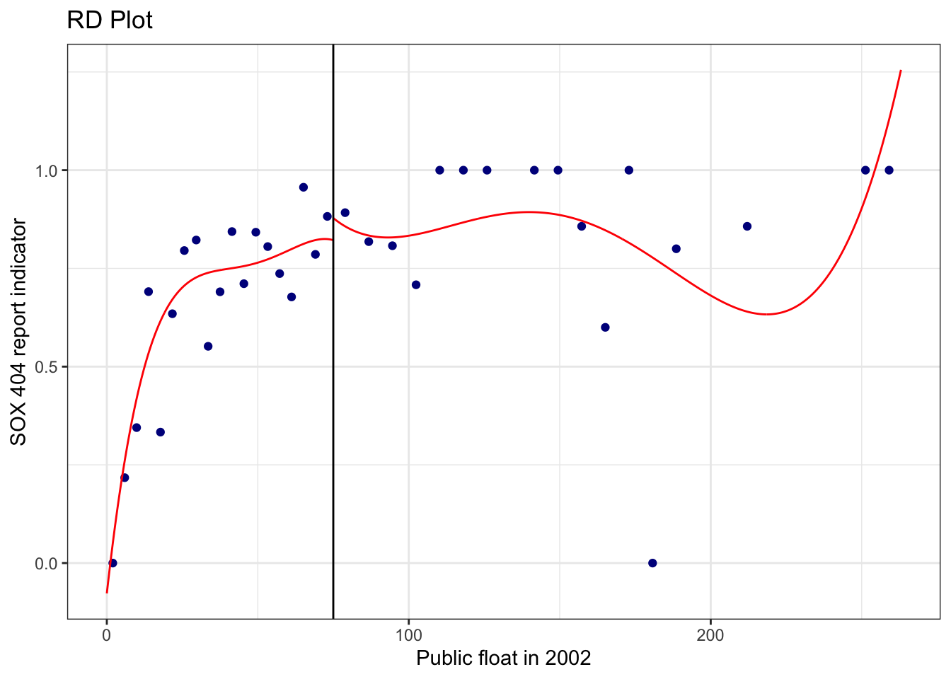
What we observe in Figure 22.1 is that, in contrast to Figure 1 of Hoekstra (2009), there is no obvious discontinuity in the probability of treatment (sox) around the cutoff, undermining the notion that float2002 is a viable instrument for sox.
What happens if we use float2004 as the partitioning variable?
rdplot(reg_data_fs$sox, reg_data_fs$float2004, c = cutoff,
       masspoints = "off")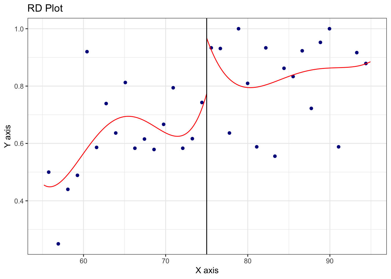
From Figure 22.2, we see that things now look a little better and we confirm this statistically next:
Sharp RD estimates using local polynomial regression.

Number of Obs.                  866
BW type                       mserd
Kernel                   Triangular
VCE method                       NN

Number of Obs.                  479          387
Eff. Number of Obs.             193          154
Order est. (p)                    1            1
Order bias  (q)                   2            2
BW est. (h)                   6.988        6.988
BW bias (b)                  10.036       10.036
rho (h/b)                     0.696        0.696

=====================================================================
                   Point    Robust Inference
                Estimate         z     P>|z|      [ 95% C.I. ]
---------------------------------------------------------------------
     RD Effect     0.241     3.273     0.001     [0.100 , 0.400]
=====================================================================
The probability jump at the cutoff is \(0.241\) with a standard error of \(0.065\). This suggests we might run fuzzy RDD with float2004 as the running variable (we defer concerns about the appropriateness of this to the discussion questions). We can do this using rdrobust() as follows:
Fuzzy RD estimates using local polynomial regression.

Number of Obs.                  866
BW type                       mserd
Kernel                   Triangular
VCE method                       NN

Number of Obs.                  479          387
Eff. Number of Obs.             211          169
Order est. (p)                    1            1
Order bias  (q)                   2            2
BW est. (h)                   7.834        7.834
BW bias (b)                  11.961       11.961
rho (h/b)                     0.655        0.655

First-stage estimates.

=====================================================================
                   Point    Robust Inference
                Estimate         z     P>|z|      [ 95% C.I. ]
=====================================================================
     Rd Effect     0.240     3.412     0.001     [0.106 , 0.392]
=====================================================================

Treatment effect estimates.

=====================================================================
                   Point    Robust Inference
                Estimate         z     P>|z|      [ 95% C.I. ]
---------------------------------------------------------------------
     RD Effect    -0.746    -0.802     0.423    [-2.176 , 0.912]
=====================================================================
The estimated effect at the cutoff is \(-0.746\), which is not significantly different from zero.
We can also run a kind of intent-to-treat RDD as follows and can also plot this as in Figure 22.3.
Sharp RD estimates using local polynomial regression.

Number of Obs.                  866
BW type                       mserd
Kernel                   Triangular
VCE method                       NN

Number of Obs.                  479          387
Eff. Number of Obs.             174          142
Order est. (p)                    1            1
Order bias  (q)                   2            2
BW est. (h)                   5.952        5.952
BW bias (b)                   8.546        8.546
rho (h/b)                     0.697        0.697

=====================================================================
                   Point    Robust Inference
                Estimate         z     P>|z|      [ 95% C.I. ]
---------------------------------------------------------------------
     RD Effect    -0.202    -0.960     0.337    [-0.601 , 0.206]
=====================================================================rdplot(reg_data_fs$risk_asymm, reg_data_fs$float2004,
c = cutoff, masspoints = "off")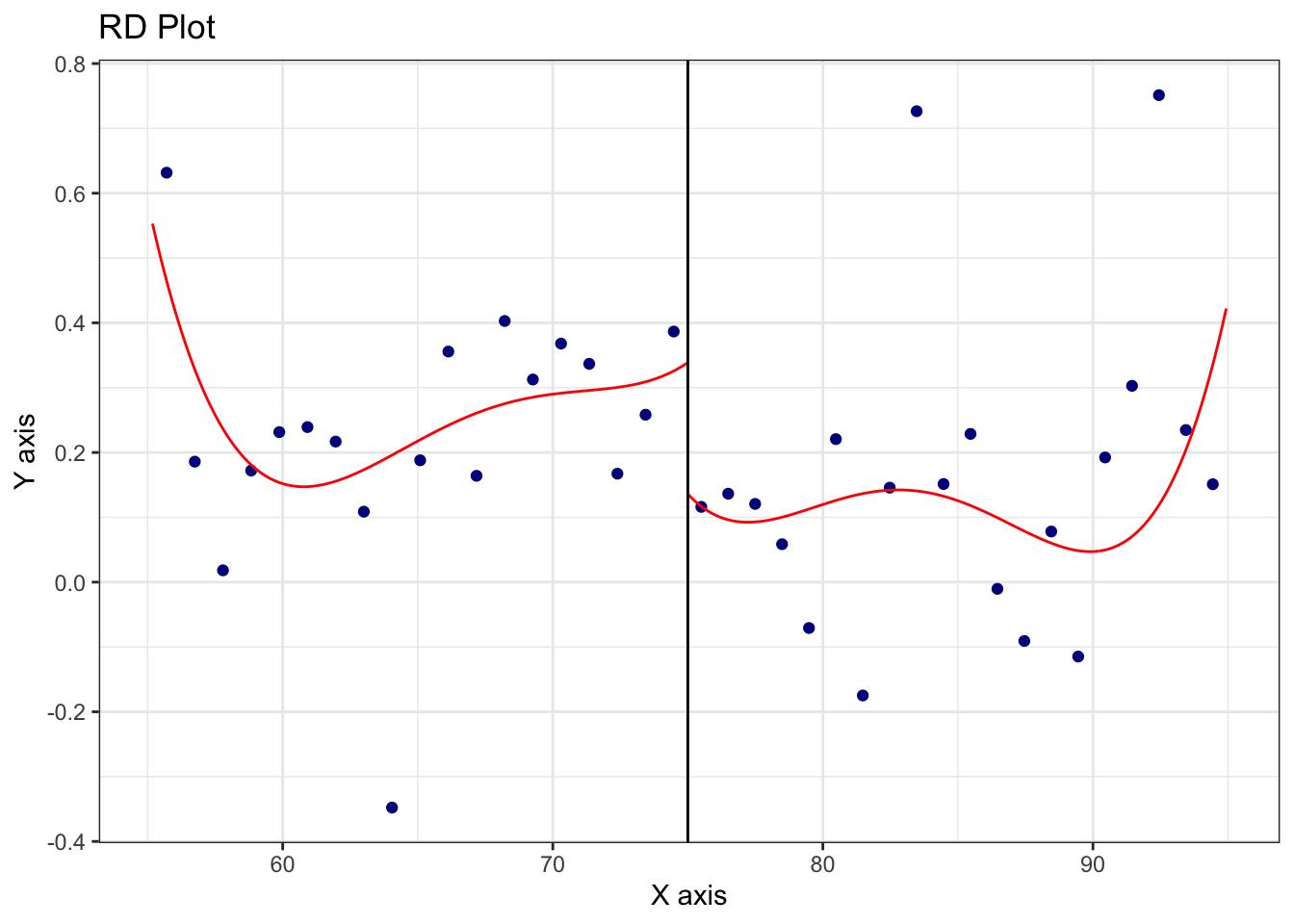
However, in neither the fuzzy RDD nor the intent-to-treat RDD do we reject the null hypothesis of no effect of SOX on risk asymmetry.10
22.5 RDD in accounting research
While RDD has seen an explosion in popularity since the turn of the century, relatively few papers in accounting research have used it. Armstrong et al. (2022) identify seven papers using RDD (which they flag as 5% of papers using what they term “quasi-experimental methods”) and we identify an additional five papers not included in their survey, suggesting that papers using RDD represent less than 1% of papers published in top accounting journals since 1999. In this subsection, we examine each of these papers, most of which fall into one of the categories below, to illustrate and discuss how RDD is used in practice in accounting research.
22.5.1 Quasi-RDD
In some settings, RDD would appear to be applicable because there is sharp assignment to treatment based on the realization of a continuous running variable exceeding a pre-determined threshold. For example, debt covenants are often based on accounting-related variables that are continuous, but covenant violation is a discontinuous function of those variables. In this setting, manipulation of the running variable would be one issue (e.g., firms may manage earnings to avoid costly covenant violations). But a bigger issue in practice is that the running variables are difficult to measure precisely (e.g., many covenants use ratios that are not defined in terms of standard accounting variables) and the thresholds are often not easily observed (e.g., covenants that change over time in ways that are difficult for a researcher to capture precisely).
As a result, papers that claim to be “using a regression discontinuity design” (e.g., p. 2114 of Chava and Roberts, 2008) simply regress the outcome of interest on a treatment indicator and some controls, perhaps restricting the sample to observations closer to violating covenants. While some have called this quasi-RDD, this is arguably simply not-RDD.
In accounting research, Tan (2013) and Vashishtha (2014) fall into this category because of data constraints. In contrast, we saw above there was no data impediment to using RDD in Bloomfield (2021).
22.5.2 Russell 1000/2000 and stuff (mostly taxes)
Another popular area applying RDD is the burgeoning literature studying the effect of institutional ownership on effective tax rates. Khan et al. (2016), Chen et al. (2019), and Bird and Karolyi (2017) exploit the discontinuous relationship between market capitalization and assignment to either the Russell 1000 or the Russell 2000 index to test for the effect of institutional ownership on tax planning. These papers build on the setting studied earlier in Boone and White (2015) (see discussion questions below).
Unfortunately, subsequent research (e.g., Appel et al., 2024) shows that the data on index assignments supplied by Russell yielded significant differences in pre-treatment outcome variables on either side of the notional discontinuity going from 1,000 to 1,001 in the rank of market capitalization. Young (2018) even shows that this year’s “plausibly exogenous” index assignment actually “causes” lower tax rates in past years, violating the laws of causation and suggesting that the results in Bird and Karolyi (2017) are spurious (Bird and Karolyi, 2017 was later retracted by The Accounting Review).
Another paper using the Russell 1000/2000 setting is Lin et al. (2017), which relates index assignment to “increases [in] industry peers’ likelihood and frequency of issuing management forecasts” (emphasis added).
22.5.3 Other papers using RDD
Kajüter et al. (2018) and Manchiraju and Rajgopal (2017) use RDD in the context of event studies of the classic capital-market kind. Manchiraju and Rajgopal (2017) is covered in the discussion questions below, so we will briefly discuss just Kajüter et al. (2018) here.
Kajüter et al. (2018) “exploit a regulatory change in Singapore to analyze the capital market effects of mandatory quarterly reporting. The listing rule implemented in 2003 has required firms with a market capitalization above S$75 million—but not firms with a market capitalization below this threshold—to publish quarterly financial statements.” The main analyses of Kajüter et al. (2018) appear to be those in Table 3 (univariate analysis) and Table 4 (polynomial regressions). Given that analysis for Table 3 has only 54 observations (25 of which were treatment firms), overly sophisticated analyses may have asked too much of the data, but the authors do include a sensitivity of the estimated effect to alternative bandwidths in Figure 2. So, it is not clear why the authors do not provide a plot of the underlying 54 data points (given the size of the data set, it could have been supplied as a table).
Two additional papers in accounting research apply RDD in corporate governance settings. Armstrong et al. (2013) also use RDD to evaluate the effectiveness of stock-based compensation plans being voted down but report no statistically significant effects of the treatment in their setting. Ertimur et al. (2015) examine the market reaction to shareholder votes that provide majority support for switching from a plurality voting standard for directors to the more stringent majority voting standard and we provide some discussion questions related to this paper below.
Finally, Figure 1 of Li et al. (2018), which we covered in Chapter 21, presents RDD plots and we include some discussion questions on this analysis below.
22.6 Further reading
As discussed above, this chapter is intended to complement existing materials, and we focus more on practical issues and applications in accounting research. The quality of pedagogical materials for RDD is high. Lee and Lemieux (2010) remains an excellent reference as is Chapter 6 of Angrist and Pischke (2008). Chapter 6 of Cunningham (2021) and Chapter 20 of Huntington-Klein (2021) cover RDD.
22.7 Discussion questions
There are many discussion questions below and we expect that instructors will only assign a subset of these. You should read enough of the papers to be able to answer questions you have been assigned below.
22.7.1 Hoekstra (2009)
What is the treatment in Hoekstra (2009)? What alternative (control) is it being compared with? Is identifying the “treatment” received by the control group always as difficult as it is in Hoekstra (2009)? Provide examples from other papers or settings in your answer.
Which approach makes the most sense in Hoekstra (2009)? Sharp RDD? Or fuzzy RDD? Why?
RDD inherently estimates a “local” treatment effect. Which group of potential students is the focus of Hoekstra (2009)? Can you think of other groups that we might be interested in learning more about? How might the actual treatment effects for those groups differ and why?
22.7.2 Bloomfield (2021)
- Compare the data in
iliev_2010andfloat_data(as used in Bloomfield (2021)) for the two firms shown in the output below. What choices has Bloomfield (2021) made in processing the data for these two firms? Do these choices seem to be the best ones? If not, what alternative approach could be used?
iliev_2010 |>
filter(gvkey == "001728")| gvkey | fyear | fdate | pfdate | pfyear | publicfloat | mr | af | cik |
|---|---|---|---|---|---|---|---|---|
| 001728 | 2001 | 2001-12-31 | 2002-03-01 | 2002 | 96.9818 | FALSE | FALSE | 225051 |
| 001728 | 2002 | 2002-12-31 | 2002-06-28 | 2002 | 69.0750 | FALSE | FALSE | 225051 |
| 001728 | 2003 | 2003-12-31 | 2003-06-27 | 2003 | 71.2024 | FALSE | FALSE | 225051 |
| 001728 | 2005 | 2005-01-01 | 2004-07-03 | 2004 | 105.8267 | TRUE | TRUE | 225051 |
| 001728 | 2005 | 2005-12-31 | 2005-07-01 | 2005 | 87.1456 | TRUE | TRUE | 225051 |
float_data |>
filter(gvkey == "001728")| gvkey | float2004 | float2002 |
|---|---|---|
| 001728 | NA | 83.0284 |
iliev_2010 |>
filter(gvkey == "028712")| gvkey | fyear | fdate | pfdate | pfyear | publicfloat | mr | af | cik |
|---|---|---|---|---|---|---|---|---|
| 028712 | 2001 | 2001-12-31 | 2002-03-21 | 2002 | 21.523 | FALSE | FALSE | 908598 |
| 028712 | 2002 | 2002-12-31 | 2002-06-28 | 2002 | 11.460 | FALSE | FALSE | 908598 |
| 028712 | 2003 | 2003-12-31 | 2003-06-30 | 2003 | 13.931 | FALSE | FALSE | 908598 |
| 028712 | 2004 | 2004-12-31 | 2004-06-30 | 2004 | 68.161 | FALSE | FALSE | 908598 |
| 028712 | 2005 | 2005-12-31 | 2005-06-30 | 2005 | 26.437 | FALSE | FALSE | 908598 |
float_data |>
filter(gvkey == "028712")| gvkey | float2004 | float2002 |
|---|---|---|
| 028712 | 68.161 | 16.4915 |
The code
treat = coalesce(float2002 >= cutoff, TRUE)above is intended to replicate Stata code used by Bloomfield (2021):generate treat = float2002 >= 75.11 Why does the R code appear to be more complex? What does Stata do that R does not do? (Hint: If you don’t have access to Stata, you may find Stata’s documentation helpful.)Bloomfield (2021)’s Stata code for the
postindicator readsgenerate post = fyear - (fyr > 5 & fyr < 11) >= 2005, wherefyearis fiscal year from Compustat (see Section 14.1) andfyrrepresents the month of the fiscal-year end (e.g., May would be5).12 The code above setspost = datadate >= "2005-11-01". Are the two approaches equivalent? Do we seem to get the right values frompostusing either approach?In the text of the paper, Bloomfield (2021) claims to “use firms’ 2002 public floats … as an instrument for whether or not the firm will become treated” and to “follow Iliev’s [2010] regression discontinuity methodology”. Evaluate each of these claims, providing evidence to support your position.
Bloomfield (2021), inspired by Iliev (2010), uses
float2002rather thanfloat2004as the running variable for treatment. What issues would you be concerned about withfloat2004that might be addressed usingfloat2002? Provide some evidence to test your concerns. (Hint: Iliev (2010) uses plots, McCrary (2008) suggests some tests.) What implications do you see for the fuzzy RDD analysis we ran above usingfloat2004as the running variable?Why do you think Bloomfield (2021) did not include RDD analyses along the lines of the ones we have done above in his paper?
In Table 4, Bloomfield (2021, p. 884) uses “a difference-in-differences design to identify the causal effect of reporting flexibility on risk asymmetry.” As we say in Chapter 21, a difference-in-differences estimator adjusts differences in post-treatment outcome values by subtracting differences in pre-treatment outcome values. Why might differences in pre-treatment outcome values between observations on either side of the threshold be particularly problematic in RDD? Does the use of firm and year fixed effects (as Bloomfield (2021) does in Table 4) address this problem? Or does it just suppress it?
22.7.3 Boone and White (2015)
What is the treatment in Boone and White (2015)? (Hint: Read the title.) Most of the analyses in the paper use a “sharp RD methodology” (see Section 4). Does this make sense given the treatment? Why or why not?
In Section 5, Boone and White (2015) suggest that while “pre-index assignment firm characteristics are similar around the threshold, one concern is that there could be differences in other unobservable firm factors, leading to a violation of the necessary assumptions for the sharp RD methodology.” Is the absence of “differences in other unobservable firm factors” the requirement for sharp (rather than fuzzy) RD?
What implications, if any, does the discussion on pp. 94–95 of Bebchuk et al. (2017) have for the arguments of Boone and White (2015)?
What is the treatment variable implied by the specification in Equation (1) in Boone and White (2015)?
22.7.4 Manchiraju and Rajgopal (2017)
22.7.5 Ertimur et al. (2015)
Consider Figure 3. How persuasive do you find this plot as evidence of a significant market reaction to majority support in shareholder proposals on majority voting? What aspects of the plot do you find persuasive or unpersuasive?
If shareholders react to successful shareholder proposals on majority voting so positively, why do so many shareholders vote against such proposals (e.g., a proposal that gets 51% support has 49% of shareholders voting against it)?
Ertimur et al. (2015, p. 38) say “our analyses suggest that high votes withheld do not increase the likelihood of a director losing their seat but often cause boards to respond to the governance problems underlying the vote, suggesting that perhaps director elections are viewed by shareholders as a means to obtain specific governance changes rather than a channel to remove a director.” How do you interpret this statement? Do you find it convincing?
22.7.6 Li et al. (2018)
Figure 1 of Li et al. (2018) presents RDD plots. How does the running variable in Figure 1 differ from that in other RDD analyses you have seen? What would you expect to be the relation between the running variable and the outcome variable? Would this vary from the left to the right of the cutoff? Do you agree with the decision of Li et al. (2018, p. 283) to “include high-order polynomials to allow for the possibility of nonlinearity around the cut off time”?
What is the range of values of “distance to IDD adoption” reported in Figure 1? What is the range of possible values given the sample period of Li et al. (2018) and data reported in Appendix B of Li et al. (2018, p. 304)?
Li et al. (2018, p. 283) say that “the figures in both panels show a clear discontinuity at the date of IDD adoption.” Do you agree with this claim?
While Thistlethwaite and Campbell (1960) seems to be very commonly cited as an example of sharp RDD, it appears that only a minority of students who scored higher than the cutoff were awarded National Merit Scholarships, making it strictly an example where fuzzy RDD should be applied if the treatment of interest is receipt of a National Merit Scholarship.↩︎
Hoekstra (2009, p. 719) takes care to explain why this is not a concern in his setting.↩︎
Here notions about “too few” and “too many” reflect expectations given the natural distribution of data and not some evaluation of the merits of having students on one side of the cutoff or the other.↩︎
Iliev (2010, p. 1165) describes public float as “the part of equity not held by management or large shareholders, as reported on the first page of the company 10-K.” See also https://www.sec.gov/news/press/2004-158.htm.↩︎
Here “hand collection” includes using web-scraping the SEC EDGAR repository. Web-scraping might use code applying regular expressions to text, such as we saw in Chapter 9.↩︎
According to the Compustat manual, the variable
auopic, when notNA, takes the value 0 if there is “No Auditor’s Report”, 1 if “Effective (No Material Weakness)”, 2 if “Adverse (Material Weakness Exists)”, 3 if “Disclaimer (Unable to Express Opinion)”, and 4 if “Delayed Filing”: https://wrds-www.wharton.upenn.edu/data-dictionary/comp_na_daily_all/funda/auopic.↩︎We explain
truncate()in Chapter 24.↩︎We discuss winsorization and the
winsorize()function in Chapter 24.↩︎Note that Bloomfield (2021) calculates “standard errors clustered by industry and fiscal year” while we just use unclustered standard errors, as we did not collect industry data to keep things simple.↩︎
Note that we see even weaker evidence of an effect if we replace
fuzzy2004withfuzzy2002in the intent-to-treat analysis.↩︎Note that we have adapted Bloomfield (2021)’s code to reflect the variable names we use above.↩︎
Note that we have adapted Bloomfield (2021)’s code to reflect the variable names we use above.↩︎