14  Post-earnings announcement drift

In Chapter 11, we saw that the cumulative returns of “good news” firms and “bad news” firms continued to drift apart even after earnings announcements. This result was considered an anomaly as, once earnings are announced, an efficient market should quickly impound the implications of those earnings and there should be no association with subsequent excess returns. Later research expanded on Ball and Brown (1968), finding that the post-earnings announcement drift (“PEAD”) existed with more refined measures and approaches.

In this chapter, we will build some foundation concepts before more closely studying a seminal paper in the PEAD literature (Bernard and Thomas, 1989). As most of the research on PEAD has focused on quarterly earnings, we will spend some time understanding Compustat’s database of quarterly financial statement information, comp.fundq.

A core concept in PEAD research is earnings surprise, which can be defined quite generally as actual earnings minus expected earnings. Thus to measure earnings surprise, we need a measure of expected earnings. Early research used time-series models of earnings to develop earnings expectation models. We will look closely at Foster (1977), which is an early study of the behaviour of quarterly accounting data.

Tip

The code in this chapter uses the packages listed below. For instructions on how to set up your computer to use the code found in this book, see Section 1.2. Quarto templates for the exercises below are available on GitHub.

library(tidyverse)
library(DBI)
library(farr)
library(modelsummary)
library(furrr)

14.1 Fiscal years

A concept frequently encountered in accounting and finance research is the fiscal year. Most US firms have financial reporting periods ending on 31 December of each year. Most Australian firms have financial reporting periods ending on 30 June of each year, perhaps because accountants don’t want to be preparing financial statements during the summer month of January.

Some US firms (often retailers) have fiscal year-ends in January. For example, Autodesk—“a global leader in 3D design, engineering, and entertainment software and services”—had a fiscal year-end on 31 January 2021. In contrast, Akamai Technologies had a fiscal year-end ending 31 December 2020. An analyst wishing to compare financial performance of Autodesk and Akamai is likely to line up both of these periods as “fiscal 2020”.

Note that there is no standard definition of “fiscal year” in practice. Fedex describes the year ending 31 May 2020 as “fiscal 2019” and General Mills describes the same period as “fiscal 2020”.

Compustat has the variable fyear (called fyearq on comp.fundq), which is described as “fiscal year”. Before zooming in on fyear, note that there are four variables of type Date on comp.funda and these are listed in Table 14.1.

Table 14.1: Date variables on comp.funda

Variable	Description
datadate	Period-end date
apdedate	Actual period-end date
pdate	Date the data are updated on a preliminary basis
fdate	Date the data are finalized

PostgreSQL

Before proceeding further, we set up connections to the database tables that we will use in this chapter. Note that we set check_interrupts = TRUE in connecting to PostgreSQL so we can cancel a long-running query if necessary.

db <- dbConnect(RPostgres::Postgres(),
                bigint = "integer",
                check_interrupts = TRUE)

funda <- tbl(db, Id(schema = "comp", table = "funda"))
fundq <- tbl(db, Id(schema = "comp", table = "fundq"))
company <- tbl(db, Id(schema = "comp", table = "company"))

ccmxpf_lnkhist <- tbl(db, Id(schema = "crsp", table = "ccmxpf_lnkhist"))

parquet

Before proceeding further, we set up connections to the database tables that we will use in this chapter.

db <- dbConnect(duckdb::duckdb())

funda <- load_parquet(db, schema = "comp", table = "funda")
fundq <- load_parquet(db, schema = "comp", table = "fundq")
company <- load_parquet(db, schema = "comp", table = "company")

ccmxpf_lnkhist <- load_parquet(db, schema = "crsp", 
                               table = "ccmxpf_lnkhist")

We construct the same funda_mod remote data frame we saw in earlier chapters.

funda_mod <-
  funda |>
  filter(indfmt == "INDL", datafmt == "STD",
         consol == "C", popsrc == "D")

To understand the date variables on comp.funda, we focus on Apple (gvkey == "001690"), whose “fiscal year is the 52- or 53-week period that ends on the last Saturday of September”.

apple_dates <-
  funda_mod |> 
  filter(gvkey == "001690") |> 
  collect() |>
  select_if(is.Date)

While there are several date variables, it seems that data on fields other than datadate are only available for more recent periods.

apple_dates |>
  filter(!is.na(apdedate)) |>
  head()

# A tibble: 6 × 4
  datadate   apdedate   fdate      pdate     
  <date>     <date>     <date>     <date>    
1 2003-09-30 2003-09-27 NA         NA        
2 2004-09-30 2004-09-25 NA         NA        
3 2005-09-30 2005-09-24 NA         NA        
4 2006-09-30 2006-09-30 2007-01-01 2006-10-18
5 2007-09-30 2007-09-29 2007-11-16 2007-10-22
6 2008-09-30 2008-09-27 2008-11-05 2008-10-21

In its 10-K filing for 2019, Apple says “the Company’s fiscal years 2019 and 2018 spanned 52 weeks each, whereas fiscal year 2017 included 53 weeks. A 14th week was included in the first quarter of 2017, as is done every five or six years, to realign the Company’s fiscal quarters with calendar quarters.” We also see that datadate is the last day of the month in which the period ended (apdedate).

These facts are evident in the following:

apple_dates |> 
  arrange(datadate) |>
  mutate(fyear_length = apdedate - lag(apdedate)) |>
  tail() 

# A tibble: 6 × 5
  datadate   apdedate   fdate      pdate      fyear_length
  <date>     <date>     <date>     <date>     <drtn>      
1 2019-09-30 2019-09-28 2019-11-04 2019-10-30 364 days    
2 2020-09-30 2020-09-26 2020-11-02 2020-10-29 364 days    
3 2021-09-30 2021-09-25 2021-11-01 2021-10-28 364 days    
4 2022-09-30 2022-09-24 2022-10-31 2022-10-27 364 days    
5 2023-09-30 2023-09-30 2023-11-04 2023-11-02 371 days    
6 2024-09-30 2024-09-28 2024-11-05 2024-10-31 364 days    

(The output above notes that fyear_length has type drtn, which is an abbreviation of “duration”. The type of variable that results from subtracting one Date object from another is a difftime, which is a class of durations. See here for more details.)

While Compustat’s documentation explains how fyear is determined, many database providers do not adequately explain variables, so being able to infer what an item describes is a useful skill. To help build this skill, we will try to deduce what fyear means here without reading the manual. We will figure out fyear by collecting data from Compustat on fyear and datadate, and then doing some statistical and graphical analysis of these data. As a side effect, we will also reinforce some aspects of regression analysis using R that we learnt about in Chapter 3.

We begin by collecting all combinations of fyear and datadate found on comp.funda and extracting the month and year applicable to each of these.

fyear_data <-
  funda_mod |>
  distinct(fyear, datadate) |>
  mutate(month = month(datadate),
         year = year(datadate)) |>
  filter(!is.na(fyear)) |>
  collect() 

We then run a couple of regression models on the data (the discussion questions below will explore these in more detail).

fms <- list(lm(fyear ~ factor(month) + year - 1, data = fyear_data),
            lm(fyear ~ month + year, data = fyear_data))

The results of these regressions are shown in Table 14.2.

modelsummary(fms,
             estimate = "{estimate}",
             statistic = NULL, 
             align = "ldd",
             gof_map = "r.squared")

Table 14.2: Regression of fyear on month indicators

	(1)	(2)
factor(month)1	-1.000
factor(month)2	-1.000
factor(month)3	-1.000
factor(month)4	-1.000
factor(month)5	-1.000
factor(month)6	0.000
factor(month)7	0.000
factor(month)8	0.000
factor(month)9	0.000
factor(month)10	0.000
factor(month)11	0.000
factor(month)12	0.000
year	1.000	1.000
(Intercept)		-1.082
month		0.122
R2	1.000	1.000

Having run the regressions, we can add the fitted values for each model to the data set.

fyear_plot_data <-
  fyear_data |>
  mutate(pred_1 = predict(fms[[1]]), 
         pred_2 = predict(fms[[2]]),
         resid_1 = pred_1 - fyear,
         resid_2 = pred_2 - fyear)

Finally we take a sample from fyear_plot_data to make Figure 14.1.

fyear_plot_data |>
  filter(year %in% c(2001, 2002)) |>
  select(datadate, fyear, pred_1, pred_2) |>
  distinct() |>
  arrange(datadate) |>
  ggplot(aes(x = datadate)) +
  geom_point(aes(y = fyear, color = "fyear")) +
  geom_line(aes(y = pred_1, color = "pred_1")) +
  geom_line(aes(y = pred_2, color = "pred_2")) +
  scale_x_date(date_breaks = "1 month") + 
  theme(axis.text.x = element_text(angle = 90),
        legend.position = "inside", legend.position.inside = c(.85, .35))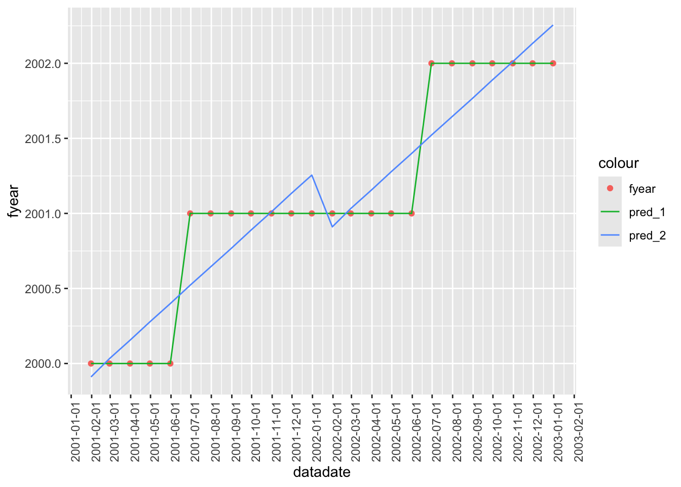

Figure 14.1: Plot of fyear against datadate for sample values

14.1.1 Exercises

1. What is different between the first and second models in fms? What is factor() doing here?

2. What does the inclusion of - 1 do in the first model in fms? Would the omission of - 1 affect the fit of that model? Would it affect the interpretability of results? Would the inclusion of - 1 affect the fit of the second model in fms? Would it affect the interpretability of results?

3. Does Figure 14.1 help you understand what’s going on? Why did we focus on a relatively short period in Figure 14.1? (Hint: What happens if you remove the line filter(year %in% c(2001, 2002)) |> from the code?)

4. Using year and month, add some code along the lines of mutate(fyear_calc = ...) to calculate fyear. Use this code to create a function fiscal_year(datadate). Check that you match fyear in each case.

14.2 Quarterly data

In Chapters 6 and 8, we focused on annual data from Compustat. But for many purposes, we will want to use quarterly data. While Ball and Brown (1968) used annual data, the PEAD literature has generally focused on quarterly data.

We begin by creating fundq_mod, the quarterly analogue of funda_mod.

fundq_mod <-
  fundq |>
  filter(indfmt == "INDL", datafmt == "STD", consol == "C", popsrc == "D")

In Chapter 6, we saw that, by focusing on the “standard” subset of observations, we have (gvkey, datadate) forming a primary key. Alas, the same is not true for quarterly data, as we can see in the output below:

fundq_mod |>
  group_by(gvkey, datadate) |>
  summarize(num_rows = n(), .groups = "drop") |>
  count(num_rows) |>
  collect()

# A tibble: 2 × 2
  num_rows       n
     <dbl>   <dbl>
1        2    1550
2        1 2041613

To dig deeper, we create the data frame fundq_probs that captures the problem cases implied by the output above.

fundq_probs <-
  fundq_mod |>
  group_by(gvkey, datadate) |>
  filter(n() > 1) |>
  ungroup() |>
  select(gvkey, datadate, fyearq, fqtr, fyr, rdq) |>
  arrange(gvkey, datadate) |>
  collect()

It turns out that the cause of the problems can be found by looking more closely at funda_mod for firms in fundq_probs around the problematic periods. One such firm is gvkey == "001224", which has observations in fundq_probs for fiscal years 2013 and 2014.

funda_mod |>
  filter(gvkey == "001224", between(fyear, 2012, 2015)) |>
  select(gvkey, datadate) |>
  arrange(gvkey, datadate) |>
  collect()

# A tibble: 4 × 2
  gvkey  datadate  
  <chr>  <date>    
1 001224 2012-12-31
2 001224 2013-12-31
3 001224 2014-09-30
4 001224 2015-09-30

In this case, the firm changed its year-end from December to September during 2014. Thus, Q4 of the year ending 2013-12-31 became Q1 of the year ending 2014-09-30. Compustat retains the data for the quarter ending 2013-12-31 twice: once as Q4 and once as Q1.

Meanwhile, Q1 of what would have been the year ending 2014-12-31 became Q2 of the year ending 2014-09-30.¹ But there is no year ending 2014-12-31 on comp.funda for this firm, so Compustat sets fqtr to NA for the second row of data for the quarter ending 2014-03-31, as can be seen in the following:

fundq_probs |>
  filter(gvkey == "001224") |>
  arrange(gvkey, datadate, fqtr)

# A tibble: 6 × 6
  gvkey  datadate   fyearq  fqtr   fyr rdq       
  <chr>  <date>      <int> <int> <int> <date>    
1 001224 2013-12-31   2014     1     9 2014-02-11
2 001224 2013-12-31   2013     4    12 2014-02-11
3 001224 2014-03-31   2014     2     9 2014-04-30
4 001224 2014-03-31   2014    NA    12 2014-04-30
5 001224 2014-06-30   2014     3     9 2014-08-11
6 001224 2014-06-30   2014    NA    12 2014-08-11

So, the variable fyr allows us to distinguish rows and, from the following analysis, we see that (gvkey, datadate, fyr) is a valid primary key for the “standard” subset of comp.fundq.

fundq_mod |>
  count(gvkey, datadate, fyr, name = "num_rows") |>
  count(num_rows) |>
  collect()

# A tibble: 1 × 2
  num_rows       n
     <dbl>   <dbl>
1        1 2044713

fundq_mod |>
  select(gvkey, datadate, fyr) |>
  mutate(across(everything(), is.na)) |>
  filter(if_any(everything())) |>
  count() |>
  pull()

[1] 0

Presumably the idea is to allow researchers to link data from comp.funda with data from comp.funda. Using fyr and fyear, we can recover the relevant annual datadate.

link_table <-
  fundq_mod |> 
  rename(datadateq = datadate) |>
  select(gvkey:fyr) |>
  mutate(year = if_else(fyr <= 5L, fyearq + 1L, fyearq)) |>
  mutate(month = lpad(as.character(fyr), 2L, "0")) |>
  mutate(datadate = as.Date(str_c(year, month, '01', sep = "-"))) |>
  mutate(datadate = as.Date(datadate + months(1) - days(1))) |>
  select(-month, -year, -fqtr) |>
  collect()

link_table |>
  arrange(gvkey, datadateq) 

# A tibble: 2,044,713 × 5
   gvkey  datadateq  fyearq   fyr datadate  
   <chr>  <date>      <int> <int> <date>    
 1 001000 1966-03-31   1966    12 1966-12-31
 2 001000 1966-06-30   1966    12 1966-12-31
 3 001000 1966-09-30   1966    12 1966-12-31
 4 001000 1966-12-31   1966    12 1966-12-31
 5 001000 1967-03-31   1967    12 1967-12-31
 6 001000 1967-06-30   1967    12 1967-12-31
 7 001000 1967-09-30   1967    12 1967-12-31
 8 001000 1967-12-31   1967    12 1967-12-31
 9 001000 1968-03-31   1968    12 1968-12-31
10 001000 1968-06-30   1968    12 1968-12-31
# ℹ 2,044,703 more rows

We could then link the table above with (gvkey, datadate) combinations from comp.funda and (gvkey, datadateq, fyr) combinations from comp.fundq (we rename datadate on comp.fundq to “datadateq” to avoid a clash between annual and quarter period-ends for any given quarter).

14.2.1 Exercises

1. Pick a couple of gvkey values from fundq_probs. Is it possible to construct a “clean” sequence of consecutive quarterly earnings announcements for each of these firms? (Here “clean” means that, at the very least, each quarter shows up just once in the series.) What challenges does one face in this task?

2. The code below produces Figure 14.2. From Figure 14.2, it seems that Q2 has been the most profitable on average over the last three decades, while in all decades, Q4 has seen the most sales. Can you speculate as to what might explain these facts?

ni_annual <-
  funda_mod |>
  select(gvkey, datadate, fyr, sale, ni) |>
  collect()

ni_qtrly <-
  fundq_mod |>
  select(gvkey, datadate, fyr, fqtr, saleq, niq, ibq) |>
  rename(datadateq = datadate) |>
  collect()

ni_merged <-
  ni_annual |>
  inner_join(link_table, by = c("gvkey", "datadate", "fyr")) |>
  inner_join(ni_qtrly, by = c("gvkey", "fyr", "datadateq"))

plot_data <-
  ni_merged |> 
  mutate(decade = str_c(floor(fyearq / 10) * 10, "s")) |>
  filter(!is.na(fqtr), fyearq < 2020) |>
  group_by(decade, fqtr) |> 
  summarize(prop_ni = sum(niq, na.rm = TRUE)/
              sum(ni, na.rm = TRUE),
            prop_sale = sum(saleq, na.rm = TRUE)/
              sum(sale, na.rm = TRUE),
            .groups = "drop") |>
  mutate(fqtr = factor(fqtr)) |>
  pivot_longer(cols = c(prop_ni, prop_sale),
               names_to = "metric",
               values_to = "value")

plot_data |>
  ggplot(aes(x = fqtr, y = value, fill = fqtr)) +
  geom_bar(stat = "identity") +
  facet_grid(metric ~ decade) +
  theme(legend.position = "none")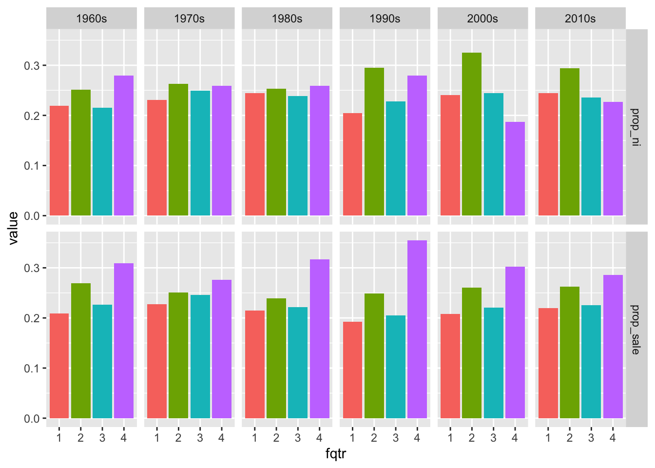

Figure 14.2: Sales and net income by quarter over decades

3. Create another plot using data in ni_merged that you think might be interesting. (Feel free to add variables to ni_annual or ni_qtrly before merging.)

14.3 Time-series properties of earnings

Foster (1977) studies the properties of quarterly accounting variables (sales, net income, and expenses) and considers the predictive ability of six models. Models 1 and 2 relate values in quarter \(Q_t\) to values in quarter \(Q_{t-4}\) and is therefore a seasonal model. Models 3 and 4 relate values in quarter \(Q_t\) to values in the adjacent quarter (\(Q_{t-1}\)). Model 5 builds on Model 2 by including a component related to \((Q_{t-1} - Q_{t-5})\). Finally, Foster (1977) considers the “Box-Jenkins time-series methodology” as Model 6.

In this section, we will do a loose replication of Foster (1977). We say “loose” because we will not try to match the sample composition or even all the details of the approach, but the basic ideas and some of the details will be the same. We replace the Box-Jenkins approach with an alternative model, as Box-Jenkins forecasting methods are more complex and not often used in accounting research today.

Foster (1977) focuses on 69 firms meeting sample-selection criteria, including the availability of quarter sales and earnings information over the period of 1946–1974. To keep our analysis to a comparable number of firms, we will choose 70 firms based on criteria detailed below. While Foster (1977) uses what he calls an “adaptive forecasting” approach whereby “all data available at the time the forecast was made were used to forecast”, we will limit ourselves to 20 quarters of data available at the time the model is developed. As a substantial majority of observations in Foster (1977) come from 12 two-digit SIC industries, we limit our sample to firms in the industries listed in Table 1 of that paper. Finally, while Foster (1977) evaluates the forecasting performance over the 1962–1974 period, we will focus on just 2 years: 1974 and 2019. These choices are implemented using the following code:

n_qtrs <- 20
n_firms <- 70
focus_years <- c(1974L, 2019L)
# See Table 1 of Foster (1977) for SICs
sic2s <- as.character(c(29, 49, 28, 35, 32, 33, 37, 20, 26, 10, 36, 59))

companies <-
  company |>
  mutate(sic2 = str_sub(sic, 1L, 2L)) |>
  filter(sic2 %in% sic2s) |>
  select(gvkey, sic2)

Our first step is to collect the data from comp.fundq that we need into a data frame that we give the name fundq_local.

fundq_local <-
  fundq_mod |>
  semi_join(companies, by = "gvkey") |>
  filter(saleq > 0 & !is.na(saleq)) |>
  select(gvkey, datadate, fyr, fqtr, fyearq, rdq, niq, saleq, ibq) |>
  rename(datadateq = datadate) |>
  collect()

Next we select firm-years available on comp.funda.

firm_years <-
  funda_mod |>
  select(gvkey, datadate) |>
  collect()

We then link firm_years to fundq_local using the link_table we created earlier.

merged_data <-
  firm_years |>
  inner_join(link_table, by = c("gvkey", "datadate")) |>
  inner_join(fundq_local, 
             by = c("gvkey", "datadateq", "fyearq", "fyr"))

We identify “regular” fiscal years, which we define as fiscal years comprising four quarters and extending over exactly a year (i.e., either 365 or 366 days).

qtr_num <-
  merged_data |> 
  group_by(gvkey, datadate) |> 
  count(name = "num_quarters") |> 
  ungroup()

regular_fyears <-
  firm_years |>
  inner_join(qtr_num, by = c("gvkey", "datadate")) |>
  group_by(gvkey) |>
  arrange(gvkey, datadate) |>
  mutate(fyear_length = datadate - lag(datadate)) |>
  ungroup() |>
  mutate(regular_year = num_quarters == 4 & 
           (is.na(fyear_length) | fyear_length %in% c(365, 366))) |>
  filter(regular_year) |>
  select(gvkey, datadate)

We next limit the sample to the regular fiscal years that we defined above and calculate the variables we need to estimate and apply the models.

reg_data <-
  merged_data |>
  semi_join(companies, copy = TRUE, by = "gvkey") |>
  semi_join(regular_fyears, by = c("gvkey", "datadate")) |>
  select(gvkey, datadateq, fyearq, rdq, niq, saleq) |>
  group_by(gvkey) |>
  arrange(datadateq) |>
  mutate(sale_lag_1 = lag(saleq, 1L),
         sale_lag_4 = lag(saleq, 4L),
         sale_lag_5 = lag(saleq, 5L),
         sale_diff = saleq - sale_lag_1,
         sale_seas_diff = saleq - sale_lag_4,
         lag_sale_seas_diff  = lag(sale_seas_diff, 1L),
         ni_lag_1 = lag(niq, 1L),
         ni_lag_4 = lag(niq, 4L),
         ni_lag_5 = lag(niq, 5L),
         ni_diff = niq - ni_lag_1,
         ni_seas_diff = niq - ni_lag_4,
         lag_ni_seas_diff  = lag(ni_seas_diff, 1L)) |>
  ungroup()

We next create a fit_model() function that estimates all six models using data from the given gvkey and the 20 quarters prior to datadateq and predicts values for datadateq for all models.

The first thing done in the function is a filter for observations that relate to the firm with the gvkey supplied as an argument to the function. Note that gvkey has two meanings in the context of the code at the point where filter() is called. First, it refers to the column of reg_data. Second, it refers to the value of the gvkey supplied as an argument to the function. It is for this reason that we use gvkey to get the first meaning and use !!gvkey as a way to get the second meaning.² (We do a similar thing for the same reason when we filter on dates.)

Having obtained data related to the firm, we split the data into train_data, the data from previous periods that we will use to estimate the models, and test_data, the data for the period that we will forecast. (Note that we exit the function and return NULL if we don’t have 20 quarters of data to train the model.)

We first estimate models 2 and 4, which require no more than estimation of a drift term (\(\delta\) in the notation of Foster, 1977), which we estimate as the mean of the respective changes over the training period.

We then create predicted values for models 1–4.

The next thing we do is fit models 5 and 6. Model 6 in Foster (1977) was based on the Box-Jenkins method. Our model 6 can be viewed as an “unconstrained” version of model 5. In model 6, we regress (in the notation of Foster, 1977) \(Q_t\) on \(Q_{t-1}\), \(Q_{t-4}\), and \(Q_{t-5}\).

In the final step, we add predicted values for models 5 and 6 to the same for models 1–4, then calculate the prediction errors and return the results of our analysis.

fit_model <- function(gvkey, datadateq) {
  
  firm_data <-
    reg_data |>
    filter(gvkey == !!gvkey)

  train_data <-
    firm_data |>
    filter(datadateq < !!datadateq) |>
    top_n(n_qtrs, datadateq)

  if (nrow(train_data) < n_qtrs) return(NULL)
  
  test_data <-
    firm_data |>
    filter(datadateq == !!datadateq)

  # Estimate models 2 & 4
  model_24 <-
    train_data |>
    group_by(gvkey) |>
    summarize(sale_diff = mean(sale_diff, na.rm = TRUE),
              ni_diff = mean(ni_diff, na.rm = TRUE),
              sale_seas_diff = mean(sale_seas_diff, na.rm = TRUE),
              ni_seas_diff = mean(ni_seas_diff, na.rm = TRUE))

  # Fit models 1, 2, 3 & 4
  df_model_1234 <-
    test_data |>
    # We drop these variables because we will replace them with 
    # their means from model_24
    select(-sale_diff, -ni_diff, -sale_seas_diff, -ni_seas_diff) |>
    inner_join(model_24, by = "gvkey") |>
    mutate(ni_m1 = ni_lag_4,
           sale_m1 = sale_lag_4,
           ni_m2 = ni_lag_4 + ni_seas_diff,
           sale_m2 = sale_lag_4 + sale_seas_diff,
           ni_m3 = ni_lag_1,
           sale_m3 = sale_lag_1,
           ni_m4 = ni_lag_1 + ni_diff,
           sale_m4 = sale_lag_1 + sale_diff)

  # Fit model 5
  sale_fm5 <- tryCatch(lm(sale_seas_diff ~ lag_sale_seas_diff, 
                          data = train_data, model = FALSE),
                       error = function(e) NULL)
  
  ni_fm5 <- tryCatch(lm(ni_seas_diff ~ lag_ni_seas_diff, 
                        data = train_data, model = FALSE), 
                     error = function(e) NULL)
  
  # Fit model 6
  sale_fm6 <- tryCatch(lm(saleq ~ sale_lag_1 + sale_lag_4 + sale_lag_5, 
                          data = train_data, model = FALSE), 
                       error = function(e) NULL)
  
  ni_fm6 <- tryCatch(lm(niq ~ ni_lag_1 + ni_lag_4 + ni_lag_5,
                        data = train_data, model = FALSE), 
                     error = function(e) NULL)
  
  if (!is.null(sale_fm5) & !is.null(ni_fm5)) {
    results <-
      df_model_1234 |>
      mutate(ni_m5 = ni_lag_4 + predict(ni_fm5, 
                                        newdata = test_data)) |>
      mutate(sale_m5 = sale_lag_4 + predict(sale_fm5, 
                                            newdata = test_data)) |>
      mutate(ni_m6 = predict(ni_fm6, newdata = test_data)) |>
      mutate(sale_m6 = predict(sale_fm6, newdata = test_data))|>
      select(gvkey, datadateq, fyearq, niq, saleq, 
             matches("(ni|sale)_m[0-9]")) |>
      pivot_longer(cols = ni_m1:sale_m6,
                   names_to = "item", values_to = "predicted") |>
      mutate(actual = if_else(str_detect(item, "^ni"), niq, saleq),
             abe = abs(predicted - actual) / predicted,
             se = abe^2 * sign(predicted)) |>
      separate(item, into = c("item", "model"), sep = "_m") |>
      select(-niq, -saleq)

    results
  }
}

Note that the calculations of abe and se above ensure that the signs of each result is the same as the sign of the denominator. This will prove useful in the approach to addressing outliers that we discuss below.

In each test period, we choose the 70 firms with the largest sales within our larger sample.

top_firms <- 
  reg_data |>
  filter(fyearq %in% focus_years) |>
  group_by(gvkey, fyearq) |>
  summarize(total_sales = sum(saleq),
            .groups = "drop") |>
  group_by(fyearq) |>
  arrange(desc(total_sales)) |>
  mutate(rank = row_number()) |>
  filter(rank <= n_firms)
  
test_years <-
  reg_data |>
  semi_join(top_firms, by = c("gvkey", "fyearq")) |>
  select(gvkey, datadateq)

We then use pmap() to apply fit_model() from above to each firm-year in test_years and store the results in results.

results <-
  pmap(test_years, fit_model) |>
  list_rbind()

Before graphing results comparable to Table 3 in Foster (1977), let’s look at the results in a less processed form. We address outliers with a fix_outliers() function.

fix_outliers <- function(x) {
  if_else(x < 0 | x > 1, 1, x)
}

Figure 14.3 provides histograms of abe based on net income for both years for all six models.

results |> 
  filter(item == "ni") |>
  filter(!is.na(abe)) |>
  mutate(abe = fix_outliers(abe)) |>
  ggplot(aes(x = abe)) + 
  geom_histogram(bins = 40) + 
  facet_grid(model ~ fyearq)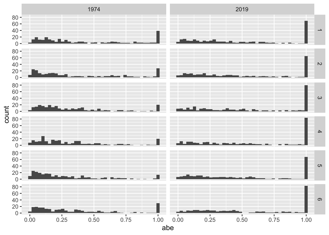

Figure 14.3: Histograms of abe

Next, we rank the models for each observation.

model_ranks <-
  results |>
  group_by(gvkey, datadateq, item) |>
  arrange(gvkey, datadateq, item, abe) |>
  mutate(rank = row_number()) |>
  group_by(fyearq, item, model) |>
  summarize(avg_rank = mean(rank, na.rm = TRUE),
            .groups = "drop") |>
  pivot_wider(names_from = c("model"), values_from = "avg_rank")

Finally, we produce results analogous to Table 3 of Foster (1977).

results_summ <-
  results |>
  mutate(abe = fix_outliers(abe),
         se = fix_outliers(se)) |>
  group_by(fyearq, item, model) |>
  summarize(mabe = mean(abe, na.rm=TRUE),
            mse = mean(se, na.rm=TRUE),
            .groups = "drop") 

We plot these results in Figure 14.4.

results_summ |>  
  pivot_longer(cols = mabe:mse, names_to = "metric", values_to = "value") |>
  ggplot(aes(x = model, y = value, fill = model)) +
  geom_bar(stat = "identity") +
  facet_grid(fyearq ~ item + metric) +
  theme(legend.position = "none")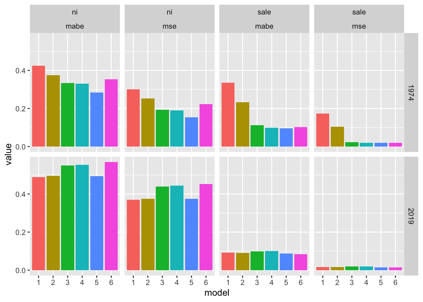

Figure 14.4: Plot of results like Table 3 of Foster (1977)

14.3.1 Exercises

1. How do the denominators in our calculations of abe and se differ from those in the analogous calculations in Foster (1977)? Is one approach to the denominator more correct than the other?

2. What does fix_outliers() do? Does Foster (1977) do anything to address outliers? If so, how does the approach in Foster (1977) compare to that of fix_outliers()? Do you agree with the approach taken in fix_outliers()? What would you do differently?

3. How do the results in Figure 14.4 compare with those in Foster (1977)?

4. What do you make of the significantly “worse” performance of models predicting ni than those predicting sale? Does this imply that ni is simply more difficult to forecast? Can you suggest an alternative approach to measuring performance that might place these models on a more “level playing field”?

14.4 Post-earnings announcement drift

The paper by Bernard and Thomas (1989) is a careful and persuasive one that rewards close reading when you have time. Bernard and Thomas (1989) build on the work of Foster et al. (1984) in measuring earnings surprise relative to expectations from Model 5 of Foster (1977); Bernard and Thomas (1989) also consider two alternative denominators.

\[ FE_i^1 = \frac{Q_{i,t} - E[Q_{i,t}]}{|Q_{i,t}|} \] \[ FE_i^2 = \frac{Q_{i,t} - E[Q_{i,t}]}{\sigma \left(Q_{i,t} - E[Q_{i,t}]\right)} \]

In the first model, \(FE_i^1\) is calculated with the absolute value of the forecast item as the denominator. In the second model, \(FE_i^2\) is calculated with the standard deviation of the forecast error as the denominator.

Rather than net income, Bernard and Thomas (1989) use “Income Before Extraordinary Items” (ibq) and we follow them in this regard. While Bernard and Thomas (1989) focus on NYSE/AMEX-listed firms, we use all firms that we can match from Compustat to CRSP.

reg_data_fos <-
  merged_data |>
  semi_join(regular_fyears, by = c("gvkey", "datadate")) |>
  select(gvkey, datadateq, fyearq, rdq, ibq) |>
  group_by(gvkey) |>
  arrange(datadateq) |>
  mutate(ib_lag_4 = lag(ibq, 4L),
         ib_seas_diff = ibq - ib_lag_4,
         lag_ib_seas_diff  = lag(ib_seas_diff, 1L),
         qtr = quarter(datadateq, with_year = TRUE)) |>
  ungroup()

Bernard and Thomas (1989) require at least 10 quarters of data to produce a forecast and use up to 24 quarters of data. If there are fewer than 16 observations, then Bernard and Thomas (1989) use the simpler Model 1 of Foster (1977). The fit_model_fos() function below is adapted from fit_model() above to reflect these features.

As before, we split the data into train_data, which we use to fit the data, and test_data, which is the holdout period for the forecast. The calculation denom_m2 provides the denominator for \(FE_i^2\).

fit_model_fos <- function(gvkey, quarter) {

  n_qtrs <- 24
  min_qtrs_fos <- 16
  min_qtrs <- 10
  
  firm_data <-
    reg_data_fos |>
    filter(gvkey == !!gvkey)

  train_data <-
    firm_data |>
    filter(qtr < !!quarter) |>
    top_n(n_qtrs, datadateq)

  test_data <-
    firm_data |>
    filter(qtr == !!quarter)

  if (nrow(train_data) < min_qtrs) return(NULL)
  if (nrow(train_data) >= min_qtrs_fos) {
    # Fit model 5
    ib_fm <- tryCatch(lm(ib_seas_diff ~ lag_ib_seas_diff, 
                         data = train_data, na.action = na.exclude,
                         model = FALSE), 
                      error = function(e) NULL)
  } else {
    ib_fm <- NULL
  }
  
  if (!is.null(ib_fm)) {
    train_results <- 
      train_data |>
      mutate(fib = ib_lag_4 + predict(ib_fm))
  } else {
    train_results <- 
      train_data |>
      mutate(fib = ib_lag_4)
  }
  
  denom_m2 <- 
    train_results |>
      mutate(fe = ibq - fib) |>
      pull() |>
      sd()
    
  if (is.null(ib_fm)) {
    results <- 
      test_data |>
      mutate(fib = ib_lag_4) 
  } else {
    results <- 
      test_data |>
      mutate(fib = ib_lag_4 + predict(ib_fm, newdata = test_data))
  }
    
  results |>
    mutate(fe1 = (ibq - fib) / abs(ibq),
           fe2 = (ibq - fib) / denom_m2)
}

So far, we have not worried about calendar time very much. But in this analysis, we are going to form portfolios each quarter based on the earnings surprise of each firm in that quarter. For this purpose, we want to measure earnings surprise in each calendar quarter. In constructing reg_data_fos above, we calculated qtr as quarter(datadateq, with_year = TRUE). The quarter() function comes from the lubridate package and, with with_year = TRUE, will return (say) the number 2014.2 if given the data 2014-06-30.

We follow Bernard and Thomas (1989) in focusing on quarters from 1974 through 1986. The following code gets a list of all quarters on the data set in that range:

quarters <-
  reg_data_fos |> 
  filter(qtr >= 1974, qtr < 1987) |>
  select(qtr) |> 
  distinct() |>
  arrange(qtr) |>
  pull()

The get_results() function calls fit_model_fos(), which produces data for a given gvkey-quarter combination, then assembles the results into a data frame and returns them.

get_results <- function(quarter) {
  
  gvkeys <- 
    reg_data_fos |>
    filter(qtr == quarter) |>
    select(gvkey) |>
    distinct() |>
    pull()
  
  map2(gvkeys, quarter, fit_model_fos) |>
    list_rbind()
}  

Warning

After setting plan(multisession), we use future_map() from the furrr package to use parallel processing. This would take much more time if we instead used map() from the purrr package. Only run this code if you want to play around with the output yourself.

The following code calls get_results() for each quarter:

plan(multisession)

results <- 
  quarters |> 
  future_map(get_results) |> 
  list_rbind() |>
  system_time()

   user  system elapsed 
  3.403   0.810  65.306 

Bernard and Thomas (1989) form portfolios based on deciles of earnings surprise. Decile 1 will have the 10% of firms with the lowest (most negative) earnings surprise. Decile 10 will have the 10% of firms with the highest (most positive) earnings surprise. But to avoid lookahead bias, the cut-offs for assigning firms to deciles will be based on the distribution of earnings surprises for the previous quarter. The get_deciles() function takes a vector of data and returns the decile cut-offs for that vector. Note that we set the highest limit to Inf, as we want to put any firms whose earnings surprise is greater than the maximum in Decile 10. Note also that we return the breaks inside a list so that the returned value can be stored in a column of a data frame, which we do in creating decile_cuts. The code creating decile_cuts is fairly self-explanatory, but note that we will be most interested in fe1_deciles_lag and fe2_deciles_lag, which are the decile cut-offs based on data from the previous quarter.

get_deciles <- function(x) {
  breaks <- quantile(x, probs = seq(from = 0, to = 1, by = 0.1),
                     na.rm = TRUE)
  breaks[length(breaks)] <- Inf
  list(breaks)
}

decile_cuts <-
  results |>
  group_by(qtr) |>
  summarize(fe1_deciles = get_deciles(fe1),
            fe2_deciles = get_deciles(fe2),
            .groups = "drop") |>
  arrange(qtr) |>
  mutate(fe1_deciles_lag = lag(fe1_deciles),
         fe2_deciles_lag = lag(fe2_deciles))

We add the decile cut-offs to the results data frame in the following code. Note that we need to use rowwise() here to calculate fe1_decile and fe2_decile row by row. While cut() is a vectorized function, it accepts just one value for the second argument breaks. However, we want to apply different breaks to each row (based on which quarter it is in). Using rowwise() allows us to do this. Once we have applied the breaks, we no longer need them, so we drop them in the last line below.

results_deciles <-
  results |>
  inner_join(decile_cuts, by = "qtr") |>
  rowwise() |>
  mutate(fe1_decile = cut(fe1, fe1_deciles_lag, labels = FALSE),
         fe2_decile = cut(fe2, fe2_deciles_lag, labels = FALSE)) |>
  filter(!is.na(fe1_decile) | !is.na(fe2_decile)) |>
  ungroup() |>
  select(-matches("^fe[12]_deciles"))

We will need to grab stock returns for our earnings announcements. The following code is more or less copy-pasted from earlier chapters.

ccm_link <-
  ccmxpf_lnkhist |>
  filter(linktype %in% c("LC", "LU", "LS"),
         linkprim %in% c("C", "P")) |>
  mutate(linkenddt = coalesce(linkenddt,
                              max(linkenddt, na.rm = TRUE))) |>
  rename(permno = lpermno) |>
  collect()
  
link_table <-
  results_deciles |>
  select(gvkey, rdq) |>
  inner_join(ccm_link, 
             join_by(gvkey, between(rdq, linkdt, linkenddt))) |>
  select(gvkey, rdq, permno)

Warning

Note that the following code chunk can take a few minutes to run. Parallel processing does not help much in this case, as the code is not written in a way to facilitate this.

rets <- 
  link_table |>
  get_event_rets(db, event_date = "rdq", 
                 win_start = -60, win_end = 60) |>
  nest_by(rdq, permno) |>
  system_time()

   user  system elapsed 
 15.202   3.790   4.111 

Finally, we calculate mean size-adjusted returns for each decile at each trading day relative to the earnings announcement. Here we basically follow the approach described in Bernard and Thomas (1989, p. 7). There are some issues implicit in these calculations that are discussed in Bernard and Thomas (1989) and covered in the discussion questions below.

Note that there are some duplicates in terms of (gvkey, rdq) on results_deciles. Many of these cases appear to be ones in which announcement of earnings from a prior quarter has been delayed, causing two quarters of earnings to be announced at the same time. It seems reasonable to attribute market reactions on those dates to the latest quarter, so we limit our data to the latest values of datadateq for each (gvkey, rdq).

plot_data <-
  results_deciles |>
  filter(!is.na(rdq)) |>
  group_by(gvkey, rdq) |>
  filter(datadateq == max(datadateq)) |>
  ungroup() |>
  mutate(decile = fe2_decile) |>
  inner_join(link_table, by = c("gvkey", "rdq")) |>
  inner_join(rets, by = c("rdq", "permno")) |>
  unnest(cols = c(data)) |>
  group_by(decile, relative_td) |>
  summarize(ar = mean(ret - decret, na.rm = TRUE), .groups = "drop") 

In Figures 14.5 and 14.6, we set abnormal returns for the first trading day to zero. Thus, Figure 14.5 depicts returns starting from day \(t-59\) and Figure 14.6 depicts returns starting from day \(t+1\). Adding a label to the last day of the series means we don’t need a legend.

plot_data |>
  filter(relative_td <= 0) |>
  filter(!is.na(decile)) |>
  mutate(decile = as.factor(decile)) |>
  mutate(first_day = relative_td == min(relative_td),
         last_day = relative_td == max(relative_td),
         ar = if_else(first_day, 0, ar),
         label = if_else(last_day, as.character(decile), NA)) |>
  select(-first_day) |>
  group_by(decile) |>
  arrange(relative_td) |>
  mutate(car = cumsum(ar)) |>
  ggplot(aes(x = relative_td, y = car, 
             group = decile, color = decile)) + 
  geom_line() +
  geom_label(aes(label = label), na.rm = TRUE) +
  theme(legend.position = "none")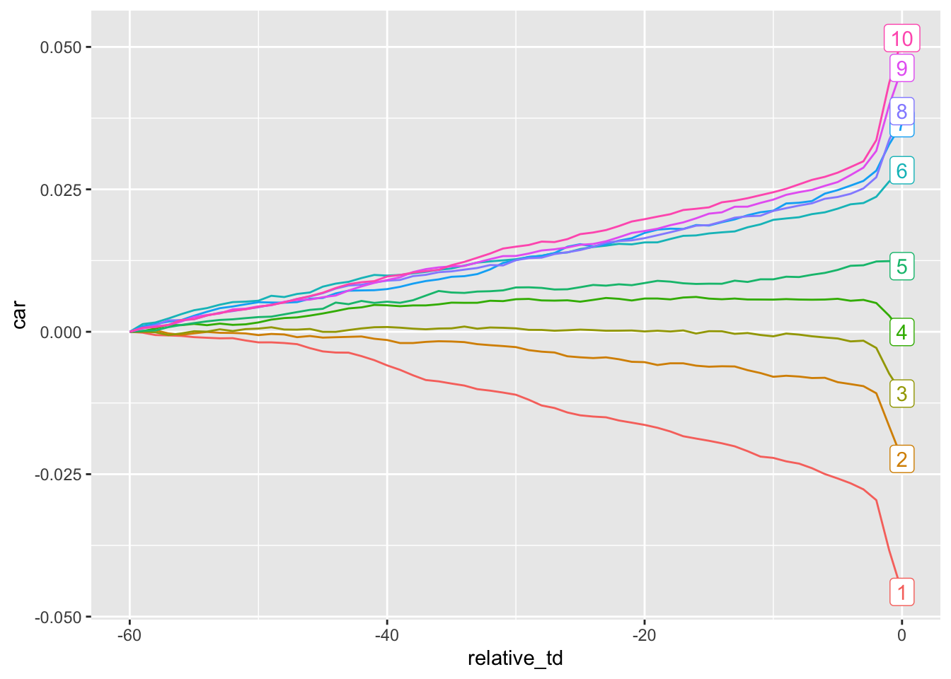

Figure 14.5: Pre-announcement returns

Figure 14.6 shows post-announcement returns for each of the ten portfolios.

plot_data |>
  filter(relative_td >= 0) |>
  filter(!is.na(decile)) |>
  mutate(decile = as.factor(decile)) |>
  mutate(first_day = relative_td == min(relative_td),
         last_day = relative_td == max(relative_td),
         ar = if_else(first_day, 0, ar),
         label = if_else(last_day, as.character(decile), NA)) |>
  group_by(decile) |>
  arrange(relative_td) |>
  mutate(car = cumsum(ar)) |>
  ggplot(aes(x = relative_td, y = car, group = decile, color = decile)) + 
  geom_line() +
  geom_label(aes(label = label), na.rm = TRUE) +
  theme(legend.position = "none")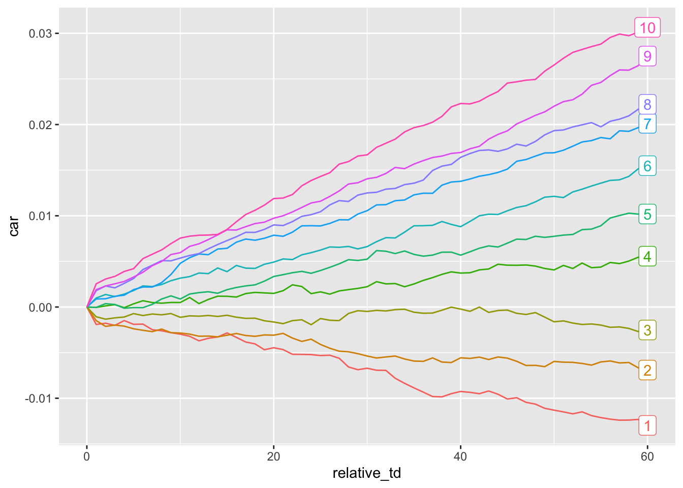

Figure 14.6: Post-announcement returns

14.4.1 Discussion questions

1. Both Bernard and Thomas (1989) and Ball and Brown (1968) were addressing issues with “conventional wisdom” at their respective times. How had conventional wisdom changed in the years between 1968 and 1989?

2. Evaluate the introduction of Bernard and Thomas (1989). How clear is the research question to you from reading this? How would you compare this introduction with other papers you have read in this course or elsewhere?

3. How persuasive do you find Bernard and Thomas (1989) to be? What evidence and arguments do you find persuasive or not persuasive? (Answering this question requires you to read the paper fairly closely.)

4. The analysis underlying Figure 14.6 considers the 13-year period from 1974 to 1986. What changes would you need to make to the code to run the analysis for the 13-year period from 2007 to 2019? (If you choose to make this change and run the code, what do you notice about the profile of returns in the post-announcement period? Does it seem necessary to make an additional tweak to the code to address this?)

5. Considering a single stock, what trading strategy is implicit in calculating ar as ret - decret?

6. In calculating mean returns by decile and relative_td (i.e., first using group_by(decile, relative_td) and then calculating ar by aggregating mean(ret - decret, na.rm = TRUE)), are we making assumptions about the trading strategy? What issues are created by this trading strategy? Can you suggest an alternative trading strategy? What changes to the code would be needed to implement this alternative?

7. Is it appropriate to add returns to get cumulative abnormal returns as is done in car = cumsum(ar)? What would be one alternative approach?

Ball, R., Brown, P., 1968. An empirical evaluation of accounting income numbers. Journal of Accounting Research 6, 159–178. https://doi.org/10.2307/2490232

Bernard, V.L., Thomas, J.K., 1989. Post-earnings-announcement drift: Delayed price response or risk premium? Journal of Accounting Research 27, 1–36. https://doi.org/10.2307/2491062

Foster, G., 1977. Quarterly accounting data: Time-series properties and predictive-ability results. The Accounting Review 52, 1–21.

Foster, G., Olsen, C., Shevlin, T., 1984. Earnings releases, anomalies, and the behavior of security returns. The Accounting Review 59, 574–603.

Wickham, H., 2019. Advanced R, second edition, Chapman & Hall/CRC The R Series. CRC Press. https://doi.org/10.1201/9781351201315

---

1. From the firm’s transitional 10-K filing at https://go.unimelb.edu.au/j7d8: “Effective September 2, 2014, the Company amended its bylaws to change the Company’s fiscal year from beginning January 1st and ending on December 31st, to beginning October 1st and ending on September 30th. As a result, this Form 10-K is a transition report and includes financial information for the period from January 1, 2014 through September 30, 2014. Subsequent to this report, the Company’s annual reports on Form 10-K will cover the fiscal year October 1st to September 30th. The period beginning January 1, 2014 through September 30, 2014 is referred to as the ‘current period’ or ‘transition period’ and the period beginning October 1, 2014 through September 30, 2015 as ‘fiscal 2015’.”

2. Chapter 19 of Wickham (2019) has more details on the “unquote” operator !!.