4 Causal inference
This is the published R edition of the book. A Python version of the book is available at era_pl_book.
The importance of causal inference in accounting research is clear from the research questions that accounting researchers seek to answer. Many questions in accounting research are causal, including examples from this book:
- Does short-selling affect firms’ level of earnings management?
- Does lowering the cost of disclosure increase the supply of disclosure?
- Do Big Four auditors increase the quality of financial statements?
- Do managerial incentives lead to managerial misstatements in financial reports?
The taxonomy for empirical research papers provided by Gow et al. (2016) comprises four categories:
- descriptive research papers
- papers focused on prediction
- papers that focus on measurement of some construct
- papers that seek—whether explicitly or not—to draw causal inferences
The survey conducted by Gow et al. (2016) suggests that most original research papers in the top three accounting research journals use observational data and that about 90% of these papers seek to draw causal inferences.
Accounting researchers’ focus on causal inference is consistent with the view that “the most interesting research in social science is about questions of cause and effect” (Angrist and Pischke, 2008, p. 3). While you may hear people talk about “interesting associations” at times, the reality is that associations (or correlations) are only interesting if there’s an interesting possible causal explanation for the associations. Associations that are mere coincidence, such as those found on the Spurious Correlations website are amusing, but unlikely to be of genuine interest to researchers or policy-makers.
At times, authors appear to disclaim any intention to draw causal inferences. Bertrand and Schoar (2003) is fairly typical: “There is no such thing as a random allocation of top executives to firms. Therefore, we are not hoping in this section to estimate the causal effect of managers on firm practices. Instead, our objective is more modest. We want to assess whether there is any evidence that firm policies systematically change with the identity of the top managers in these firms.”
There are at least two issues with this claim. First, why would anyone be interested in “evidence that firm policies systematically change with the identity of the top managers” if such changes come with no understanding as to why they change? Second, this claim is a bit of a pretence. The title of the paper is, after all, “Managing with style: The effect of managers on firm policies” and the first sentence of the abstract says “this paper investigates whether and how individual managers affect corporate behavior and performance” (emphasis added).
As another example, suppose a researcher argues that a paper that claims that “theory predicts \(X\) is associated \(Y\) and, consistent with that theory, we show \(X\) is associated with \(Y\)” is merely a descriptive paper that does not make causal inferences. However, theories are invariably causal in that they posit how exogenous variation in certain variables leads to changes in other variables. Further, by stating that “consistent with … theory, \(X\) is associated with \(Y\)”, the clear purpose is to argue that the evidence tilts the scale, however slightly, in the direction of believing the theory is a valid description of the real world: in other words, a causal inference is drawn. A paper that argues that \(Z\) is a common cause of \(X\) and \(Y\) and claims to find evidence of this is still making causal inferences (i.e., that \(Z\) causes \(X\) and \(Z\) causes \(Y\)).
Making causal inferences requires strong assumptions about the causal relations among variables. For example, as discussed below, estimating the causal effect of \(X\) on \(Y\) requires that the researcher has controlled for variables that could confound estimates of such effects.
Recently, some social scientists have argued that better research designs and statistical methods can increase the credibility of causal inferences. For example, Angrist and Pischke (2010) suggest that “empirical microeconomics has experienced a credibility revolution, with a consequent increase in policy relevance and scientific impact.” Angrist and Pischke (2010, p. 26) argue that such “improvement has come mostly from better research designs, either by virtue of outright experimentation or through the well-founded and careful implementation of quasi-experimental methods.”
The code in this chapter uses the packages listed below. For instructions on how to set up your computer to use the code found in this book, see Section 1.2 (note that Step 4 is not required for this chapter as we do not use WRDS data). Quarto templates for the exercises below are available on GitHub.
4.1 Econometrics
Empirical financial accounting research can be viewed as fundamentally a highly specialized area of applied microeconomics. Financial accounting researchers typically take classes (at some level) in microeconomics, statistics, and econometrics, either before or in parallel with more specialized classes in accounting research. This model has two significant gaps that budding researchers need to address.
The first gap is the translation of ideas from econometrics and microeconomics into what researchers do from day to day. As we will see, sometimes things get lost in this translation. One goal of this book is to reduce the gap in the domain of empirical methods.
But it’s the second gap that we want to address in this chapter, and this gap affects not only financial accounting researchers but applied economic researchers more generally. This gap is between what accounting researchers want to do, which is causal inference, and what econometrics textbooks talk about, such as consistency, unbiasedness, and asymptotic variance.1
4.1.1 What is econometrics?
Angrist and Pischke (2014, p. xi) suggest that “economists’ use of data to answer cause-and-effect questions constitutes the field of applied econometrics.” Given that “applied” here is to in contradistinction to “theoretical” econometrics, this is perhaps one working definition of econometrics for the purposes of accounting research, a field with little direct connection to the more theoretical end of econometrics. Given accounting researchers’ focus on “cause-and-effect questions” (discussed above), this definition seems consistent with what empirical accounting researchers do.
For example, we might posit that an economic phenomenon \(y\) is best modelled as follows:
\[ y = X \beta + \epsilon \tag{4.1}\]
where \(y\) and \(\epsilon\) are \(N\)-element vectors, \(X\) is an \(N \times K\) matrix, and \(\beta\) is a \(K\)-element vector of coefficients. This single-equation model “is still the workhorse in empirical economics” (Wooldridge, 2010, p. 49) and this is no doubt true in empirical accounting research.
A very important point about Equation 4.1 is that it should be viewed as a structural (causal) model. Wooldridge (2010, p. 49) writes “Goldberger (1972) defines a structural model as one representing a causal relationship, as opposed to a relationship that simply captures statistical associations. A structural equation can be obtained from an economic model, or it can be obtained through informal reasoning.”
If we were only interested in estimating this equation to generate conditional expectation function linear in the parameters, then we would not be concerned with whether \(\mathbb{E}[X \epsilon] \neq 0\), whether there were “bias” in the estimates \(\hat{\beta}\), or whether we had sufficiently “controlled for” variables in the right-hand side of the equation. Such notions only apply if we are viewing this equation as a structural model.
Viewing the equation above as a structural model, if we knew \(\beta\), we could understand how changes in \(X\) cause changes in \(y\). For example, if \(x_{ik}\) goes from \(0\) to \(1\), then we expect \(y_i\) to increase by \(\beta_k\). In other words, \(\beta_k\) can be viewed as the (causal) effect of \(x_{k}\) on \(y\). Of course, in reality, we don’t know \(\beta\); we need to estimate it using data. Much of econometrics is devoted to explaining how (and when) we can estimate \(\beta\) accurately and efficiently.
An important point to make is that, in viewing the equation above as a structural model, we depart slightly from more recent usage, which has tended to view a structural model as something deriving from an economic model, typically one starting with preferences and technologies for production of economic goods and information and deriving predictions about economic phenomena from that model. This narrower view of structural models does not seem to fit the reality that almost all empirical research proceeds without access to such models, notwithstanding a focus on causal inference.
Sometimes the reasoning behind the use of particular models is poor, and models implied by what researchers do can be poorer than they need to be. But models are always simplifications of reality and thus always in some sense “wrong”. And, even if we accept a model in a given setting, it is often the case that we “know” that our estimators are unlikely to provide unbiased estimates of the model’s true parameter values. Yet that does not change what researchers are trying to do when they conduct empirical analysis using econometric techniques.
If you look at the indexes of some standard textbooks from just a few years ago, you will see no entries for causal, causation, or similar terms.2 But we would argue that econometrics properly conceived is the social science concerned with estimation of parameters of (structural) economic models. We would further argue that any time we believe we can read off an estimate of a causal effect from an econometric analysis, we are estimating a structural model, even if the model does not involve advanced economic analysis. For example, if we randomly assign observations to treatment and control, then most would agree that we can (under certain assumptions) read causal effects off a regression of the outcome of interest on the treatment indicator. So this is a “structural” model, albeit a very simple one.
Recently, some econometric textbooks have been more explicit about causal inference as the goal of almost all empirical research in economics. One example is Mostly Harmless Econometrics (Angrist and Pischke, 2008) and another is Causal Inference: The Mixtape (Cunningham, 2021).
The definition of econometrics that we provide here is not vacuous; not everything that accounting researchers do with econometric techniques could be described as econometric analysis. At times, researchers run regressions without giving any thought as to the model they are trying to estimate. As we will see later in this book, there are settings where accounting researchers have drawn (causal) inferences from estimated coefficients about economic phenomena whose connection to the empirical models used is very far from clear. In other settings, researchers will implicitly assume that the null hypothesis implies a zero coefficient on some variable without doing any modelling of this. One of the goals of this book is to encourage researchers to keep in mind what we are trying to do when we conduct econometric analysis.
4.1.2 Econometrics: The case of conditional conservatism
Conservatism has long been regarded as a hallmark of financial reporting. Many accounting standards treat losses and gains differently, with a greater willingness to recognize losses than gains. For example, if the present value of expected future cash flows from an asset declines below the asset’s carrying value, several accounting standards (e.g., IAS 36) require the recognition of a commensurate loss. However, if the present value of expected future cash flows from an asset increases above the asset’s carrying value, those standards may defer any recognition of a gain until those future cash flows are realized. In this way, conservatism manifests as asymmetric timeliness in the recognition of losses and gains. Because this form of conservatism is conditional on news about the value of assets, it is also known as conditional conservatism.3
Basu (1997) developed a measure of asymmetric timeliness that is derived from estimation of the following regression:
\[ X_{it}/P_{it} = \alpha_0 + \alpha_1 D_{it} + \beta_0 R_{it} + \beta_1 (R_{it} \times D_{it}) + \epsilon_{it},\] where \(X_{it}\) is the earnings per share for firm \(i\) in fiscal year \(t\), \(P_{it}\) is the price per share for firm \(i\) at the beginning of fiscal year \(t\), \(R_{it}\) is the return on firm \(i\) from 9 months before fiscal year-end \(t\) to three months after fiscal year-end \(t\), and \(D_{it}\) is an indicator for \(R_{it} < 0\).
Using examples and intuition, Basu (1997) argues that \(\hat{\beta}_1\) is a measure of asymmetric timeliness. An extensive literature has exploited the Basu (1997) measure to understand the role of conservatism in accounting. For example, Ball et al. (2000, p. 22) “propose that common-law accounting income is more asymmetrically conservative than code-law, due to greater demand for timely disclosure of economic losses” and provide evidence based on differences in the Basu (1997) measure. Jayaraman and Shivakumar (2012, p. 95) “find an increase in [the Basu (1997) measure] after the passage of antitakeover laws for firms with high contracting pressures.”
This literature proceeded notwithstanding the absence of any demonstration that the Basu (1997) measure provides an unbiased and efficient estimator of an underlying conservatism parameter. While Ball et al. (2013) suggests the promise of covering the “econometrics of the Basu asymmetric timeliness coefficient” in its title, it contains little analysis of the kind seen in an econometrics text.
A more conventional econometric analysis might posit conditional conservatism as something that can be parameterized in some way. For example, specifying \(\theta\) as the key parameter—with higher values of \(\theta\) representing higher levels of conservatism—it might then be demonstrated how estimates of this underlying parameter \(\theta\) can be made—or at least how measures that are increasing in \(\theta\) can be constructed.
In an effort to establish some econometric foundations for the Basu (1997) measure, Ball et al. (2013) “model conditional conservatism as recognition of \(y\) in the current period only when it is sufficiently bad news … [and assume current period recognition] if \(y_t < c\) and zero otherwise, where \(c\) is a threshold below which current-period recognition occurs.” Focusing on the case where \(c = 0\), Ball et al. (2013) show that the expected Basu (1997) coefficient will be positive, but when there is no conditional conservatism (e.g., \(c = -\infty\) or \(c = \infty\)), the expected Basu (1997) coefficient will be zero. But Ball et al. (2013) do not even propose an underlying parameterization of conservatism on which conventional econometrics could be brought to bear. The only parameter here is \(c\), which does not have a monotonic relationship with conservatism (Ball et al., 2013 point out that both \(c = -\infty\) and \(c = \infty\) are consistent with the absence of conservatism).
In effect, Ball et al. (2013) show that if conservatism is defined as an asymmetric relationship between returns and income around zero returns, then an OLS estimator that captures an asymmetric relationship between returns and income around zero returns (such as the Basu (1997) measure) will detect conservatism.4 Ball et al. (2013, p. 1073) state that “we show that, holding other things constant, the Basu regression identifies conditional conservatism only when it exists.” Apart from the heavy lifting being done by the words “holding other things constant”, this claim belies how the Basu (1997) measure has been used in research. The two papers cited above—Ball et al. (2000) and Jayaraman and Shivakumar (2012)—interpret higher levels of the Basu (1997) measure as capturing greater conservatism. Dietrich et al. (2022, p. 2150) point out that “differences in conservatism” across firms and time “is the explicit focus of nearly all conservatism research.” But Ball et al. (2013) provide no elaboration of the concept of “greater conservatism” let alone how the Basu (1997) measure captures it.5
4.1.3 Econometrics: A brief illustration
While this is a textbook on accounting research, let’s consider a stylized example from labour economics. Suppose that we posit the following structural model:
\[ \begin{aligned} y_i &= \beta_0 + \beta_1 x_{i1} + \beta_2 x_{i2} + \beta_3 x_{i3} + \epsilon_i \\ x_{i1} &= \alpha_0 + \alpha_2 x_{i2} + \alpha_3 x_{i3} + \eta_i \end{aligned} \] where \(i\) subscripts denote individual \(i\). In the first equation, \(y_i\) is income at age 30, \(x_{i1}\) is years of education, \(x_{i2}\) is a measure of industriousness, \(x_{i3}\) is a measure of intelligence, and \(\epsilon_i\) can be interpreted as random factors that affect \(y_i\) independent of \(X_i\). In the second equation, we add coefficients, \(\alpha := \left(\alpha_0, \alpha_2, \alpha_3 \right)\), and \(\eta_i\), which can be interpreted as random factors that affect \(x_{i1}\) independent of \(x_{i2}\) and \(x_{i3}\).6
As researchers, we can postulate a model of the form above and we might obtain data on \((y, X)\) that we could use to estimate \(\beta := \left(\beta_0, \beta_1, \beta_2, \beta_3 \right)\). But we don’t know that the model is correct and even if we did, we don’t know the values in \(\beta\).
As we saw in Chapter 3, the OLS regression estimator can be written
\[ \hat{\beta} = \left(X^{\mathsf{T}}X \right)^{-1} (X^{\mathsf{T}}y) \] and it can be shown mathematically that OLS has good properties—such as unbiasedness and efficiency—under certain conditions. But in a world of cheap computing, we don’t need to break out our pencils to do mathematics. Instead, we can “play God” in some sense and fix parameter values, simulate the data, then examine how well a researcher would do in estimating the parameter values that we set.
Now we can estimate three different models and store them in a list named fms.
The results from these models are presented in Table 4.1.
modelsummary(fms,
             estimate = "{estimate}",
             statistic = NULL,
gof_map = c("nobs", "r.squared"))| (1) | (2) | (3) | |
|---|---|---|---|
| (Intercept) | 9.997 | 10.003 | 10.019 |
| education | 6.767 | 4.999 | |
| intelligence | 6.003 | 21.008 | |
| industry | 7.000 | 27.007 | |
| Num.Obs. | 100000 | 100000 | 100000 |
| R2 | 0.996 | 0.999 | 0.978 |
4.1.4 Exercises
- Looking at the simulation code, what are the true values of \(\beta := \left(\beta_0, \beta_1, \beta_2, \beta_3 \right)\) and \(\alpha := \left(\alpha_0, \alpha_1, \alpha_2 \right)\)?
- Do any of the three equations reported in Table 4.1 provide good estimates of \(\beta\)?
- Consider regression (3) in Table 4.1. With regard to the first of the two equations, are there any issues with regard to estimating \(\beta\)? What (if any) OLS assumption is violated?
- What happens if you substitute the second equation (for \(x_{i1}\)) into the first equation (for \(y_i\))? Does this equation satisfy OLS assumptions in some way?
- Using the structural equations, what happens if we arbitrarily increase the value of
industry(\(x_{i3}\)) by one unit? What happens toeducation(\(x_{i1}\))? What happens toincome(\(y_i\))? - Can you read the effect sizes from the previous question off any of the regression results in Table 4.1? If so, which one(s)?
4.2 Basic causal relations
This section provides a brief introduction to causal diagrams.
Figures 4.1–4.3 illustrate the basic ideas of causal diagrams and how they can be used to facilitate thinking about causal inference. Each figure depicts potential relationships among three observable variables. In each case, we are interested in understanding how the presence of a variable \(Z\) impacts the estimation of the causal effect of \(X\) on \(Y\). The only difference between the three graphs is the direction of the arrows linking \(Z\) with \(X\) or \(Y\). The boxes (or nodes) represent random variables and the arrows (or edges) connecting boxes represent hypothesized causal relations, with each arrow pointing from a cause to a variable assumed to be affected by it.
Pearl (2009a) shows that we can estimate the causal effect of \(X\) on \(Y\) by conditioning on a set of variables, \(Z\), that satisfies certain criteria. These criteria imply that very different conditioning strategies are needed for each of the causal diagrams (see Gow et al. (2016) for a more formal discussion).
While conditioning on variables is much like the standard notion of “controlling for” such variables in a regression, there are critical differences. First, conditioning means estimating effects for each distinct level of the set of variables in \(Z\). This concept of nonparametric conditioning on \(Z\) is more demanding than simply including \(Z\) as another regressor in a linear regression model.7 Second, the inclusion of a variable in \(Z\) may not be an appropriate conditioning strategy. Indeed, it can be that the inclusion of \(Z\) results in biased estimates of causal effects.
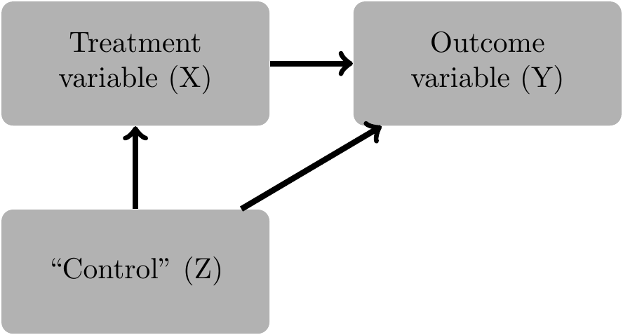
Figure 4.1 is straightforward. In this case, we need to condition on \(Z\) in order to estimate the causal effect of \(X\) on \(Y\). Note the notion of “condition on” again is more general than just including \(Z\) in a parametric (linear) model.8 The need to condition on \(Z\) arises because \(Z\) is what is known as a confounder.
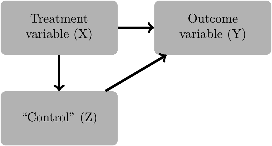
Figure 4.2 is a bit different. Here \(Z\) is a mediator of the effect of \(X\) on \(Y\). No conditioning is required in this setting to estimate the total effect of \(X\) on \(Y\). If we condition on \(X\) and \(Z\), then we obtain a different estimate, one where the “indirect effect” of \(X\) on \(Y\) via \(Z\) is captured in the coefficient on \(Z\), leaving only the “direct effect” to be reflected in the coefficient of \(X\).9

Finally in Figure 4.3, we have \(Z\) acting as what is referred to as a collider variable (Pearl, 2009b, p. 17).10 Again, not only do we not need to condition on \(Z\), but we should not condition on \(Z\) to get an estimate of the total effect of \(X\) on \(Y\). While in epidemiology, the issue of “collider bias can be just as severe as confounding” (Glymour and Greenland, 2008, p. 186), collider bias appears to receive less attention in accounting research than confounding. Many intuitive examples of collider bias involve selection or stratification. Admission to university could be a function of combined test scores (\(T\)) and interview performance (\(I\)) exceeding a threshold, i.e., \(T + I \geq C\). Even if \(T\) and \(I\) are unrelated unconditionally, a regression of \(T\) on \(I\) conditioned on admission to university is likely to show a negative relation between these two variables. To see this, we can generate some data following this simple structure.
We plot these data in Figure 4.4.
admissions |>
  ggplot(aes(x = test, y = interview, color = admitted)) +
  geom_point() +
  theme_bw()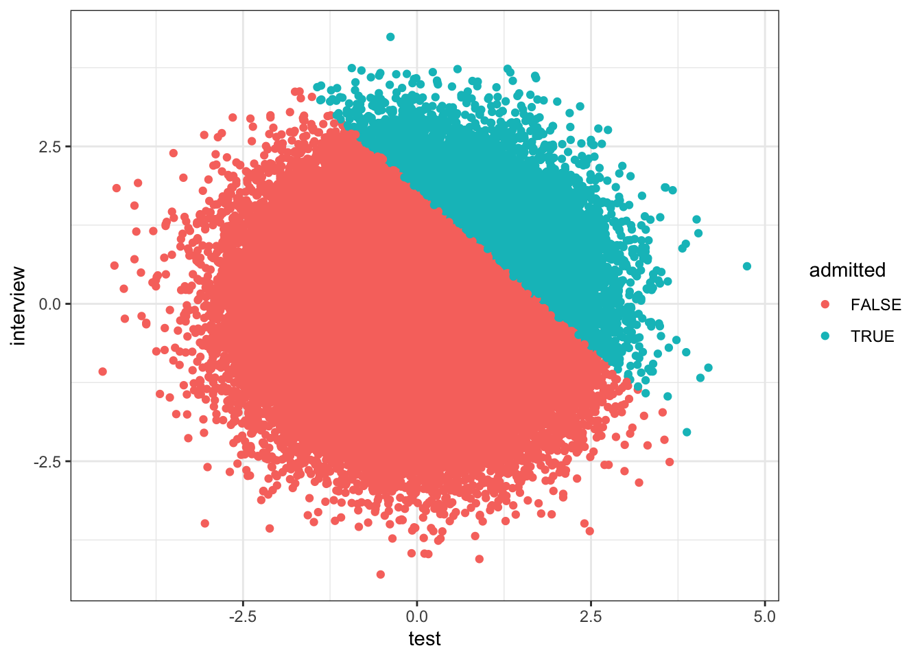
We can also fit some models to the data we have generated. In the following code, we estimate four models and store the estimated models in a list fms (for “fitted models”). Models (3) and (2) capture subsets of data where applicant are or are not admitted, respectively. Models (1) and (4) use all observations, but differ in terms of the regression terms included.
The results from these models are presented in Table 4.2.
modelsummary(fms,
             estimate = "{estimate}{stars}",
             statistic = NULL,
             gof_map = c("nobs", "r.squared"),
stars = c('*' = .1, '**' = 0.05, '***' = .01))| (1) | (2) | (3) | (4) | |
|---|---|---|---|---|
| (Intercept) | 0.001 | -0.161*** | 2.137*** | -0.161*** |
| test | -0.008*** | -0.174*** | -0.719*** | -0.174*** |
| admittedTRUE | 2.298*** | |||
| test × admittedTRUE | -0.545*** | |||
| Num.Obs. | 100000 | 90000 | 10000 | 100000 |
| R2 | 0.000 | 0.031 | 0.515 | 0.227 |
4.2.1 Exercises
- Imagine that, while you understand the basic idea that both tests and interviews affect admissions, you only have access to the regression results reported in Table 4.2. Which of the four models seems to best “describe the data”? Which of the four models seems to do worst?
- How are the coefficients reported in Table 4.2 for model (4) related to those for models (2) and (3)? Is this coincidence? Or would we always expect these relations to hold?
- As applied economists, we should be alert to the “endogeneity” of institutions. For example, if universities admitted students based on test and interview performance, they probably have good reasons for doing so. Can you think of reasons why a university might add test and interview performance into a single score? Does your story have implications for the relationship between test and interview performance?
- Using
mutate(), create a fourth variabletest_x_admittedthat is the product oftestandadmittedand run a version of model (4) in Table 4.2 that uses this variable. That is, regressinterviewontest,admitted, andtest_x_admitted. Do you get the same results as are shown above for model (4) in Table 4.2? Why or why not?
4.3 Causal diagrams: Formalities
Here we provide a brief formal treatment of some of the ideas on causal diagrams discussed above. See Pearl (2009a) for more detailed coverage.
4.3.1 Definitions and a result
We first introduce some basic definitions and a key result from Pearl (2009a). While this material may seem forbiddingly formal, the ideas are actually fairly straightforward and we will cover a few examples to demonstrate this. We recommend that in your first pass through the material, you spend just a little time on the two definitions and the theorem and then go back over them after reading the guide we provide just after the theorem.
Definition 4.1 A path \(p\) is said to be \(d\)-separated (or blocked) by a set of nodes \(Z\) if and only if
- \(p\) contains a chain \(i \rightarrow m \rightarrow j\) or a fork \(i \leftarrow m \rightarrow j\) such that the middle node \(m\) is in \(Z\), or
- \(p\) contains an inverted fork (or ) \(i \rightarrow m \leftarrow j\) such that the middle node \(m\) is not in \(Z\) and such that no descendant of \(m\) is in \(Z\).
Definition 4.2 A set of variables \(Z\) satisfies the back-door criterion relative to an ordered pair of variables \((X, Y)\) in a directed acyclic graph (DAG) \(G\) if:
- no node in \(Z\) is a descendant of \(X\); and
- \(Z\) blocks every back-door path between \(X\) and \(Y\), i.e., every such path that contains an arrow into \(X\).11
Given this criterion, Pearl (2009a, p. 79) proves the following result.
Theorem 4.1 If a set of variables \(Z\) satisfies the back-door criterion relative to \((X, Y)\), then the causal effect of \(X\) on \(Y\) is identifiable and is given by the formula \[ P(y | x) = \sum_{z} P(y | x, z) P(z), \] where \(P(y|x)\) stands for the probability that \(Y = y\), given that \(X\) is set to level \(X=x\) by external intervention.12
In plainer language, Theorem 4.1 tells us that we can estimate the causal effect of \(X\) on \(Y\) if we have a set of variables \(Z\) that satisfies the back-door criterion. Then Definition 4.2 tells us that \(Z\) needs to block all back-door paths while not containing any descendant of \(X\). Finally, Definition 4.1 tells what it means to block a path.
4.3.2 Application of back-door criterion to basic diagrams
Applying the back-door criterion to Figure 4.1 is straightforward and intuitive. The set of variables \(\{Z\}\) or simply \(Z\) satisfies the criterion, as \(Z\) is not a descendant of \(X\) and \(Z\) blocks the back-door path \(X \leftarrow Z \rightarrow Y\). So by conditioning on \(Z\), we can estimate the causal effect of \(X\) on \(Y\). This situation is a generalization of a linear model in which \(Y = X \beta + Z \gamma + \epsilon_Y\) and \(\epsilon_Y\) is independent of \(X\) and \(Z\), but \(X\) and \(Z\) are correlated. In this case, it is well known that omission of \(Z\) would result in a biased estimate of \(\beta\), the causal effect of \(X\) on \(Y\), but by including \(Z\) in the regression, we get an unbiased estimate of \(\beta\). In this situation, \(Z\) is a confounder.
Turning to Figure 4.2, \(Z\) does not satisfy the back-door criterion, because \(Z\) (a mediator) is a descendant of \(X\). However, \(\emptyset\) (i.e., the empty set) does satisfy the back-door criterion. Clearly, \(\emptyset\) contains no descendant of \(X\). Furthermore, the only path other than \(X \rightarrow Y\) that exists is \(X \rightarrow Z \rightarrow Y\), which does not have a back-door into \(X\). Note that the back-door criterion implies not only that we need not condition on \(Z\) to obtain an unbiased estimate of the causal effect of \(X\) on \(Y\), but that we should not condition on \(Z\) to get such an estimate.
Finally in Figure 4.3, we have \(Z\) acting as a collider. Again, we see that \(Z\) does not satisfy the back-door criterion because \(Z\) is a descendant of \(X\). However, \(\emptyset\) again satisfies the back-door criterion. First, it contains no descendant of \(X\). Second, the only path other than \(X \rightarrow Y\) that exists is \(X \rightarrow Z \leftarrow Y\), which does not have a back-door into \(X\). Again, the back-door criterion implies not only that we need not condition on \(Z\), but that we should not condition on \(Z\) to get an unbiased estimate of the causal effect of \(X\) on \(Y\).
4.3.3 Exercises
- Draw the DAG for the structural model above relating intelligence, industriousness, education, and income. For each \(x\) variable, identify the sets of conditioning variables that satisfy the back-door criterion with respect to estimating a causal effect of the variable on \(y\).
- For any valid set of conditioning variables not considered in Table 4.2, run regressions to confirm that these indeed deliver good estimates of causal effects.
4.4 Discrimination and bias
Let’s examine a real-world example related to possible gender discrimination in labour markets.13 When critics claimed that Google systematically underpaid its female employees, Google responded that when “location, tenure, job role, level and performance” are taken into consideration, women’s pay was basically identical to men’s. In other words, controlling for characteristics of the job, women received the same pay.
But what if stereotyping means men are given roles that are paid better? In this case, naive comparisons of wages by gender “controlling for” occupation would understate the presence of discrimination. Let’s illustrate this with a DAG based on a simple occupational sorting model with unobserved heterogeneity.
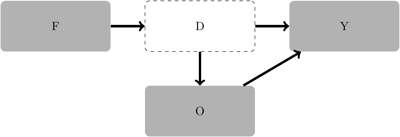
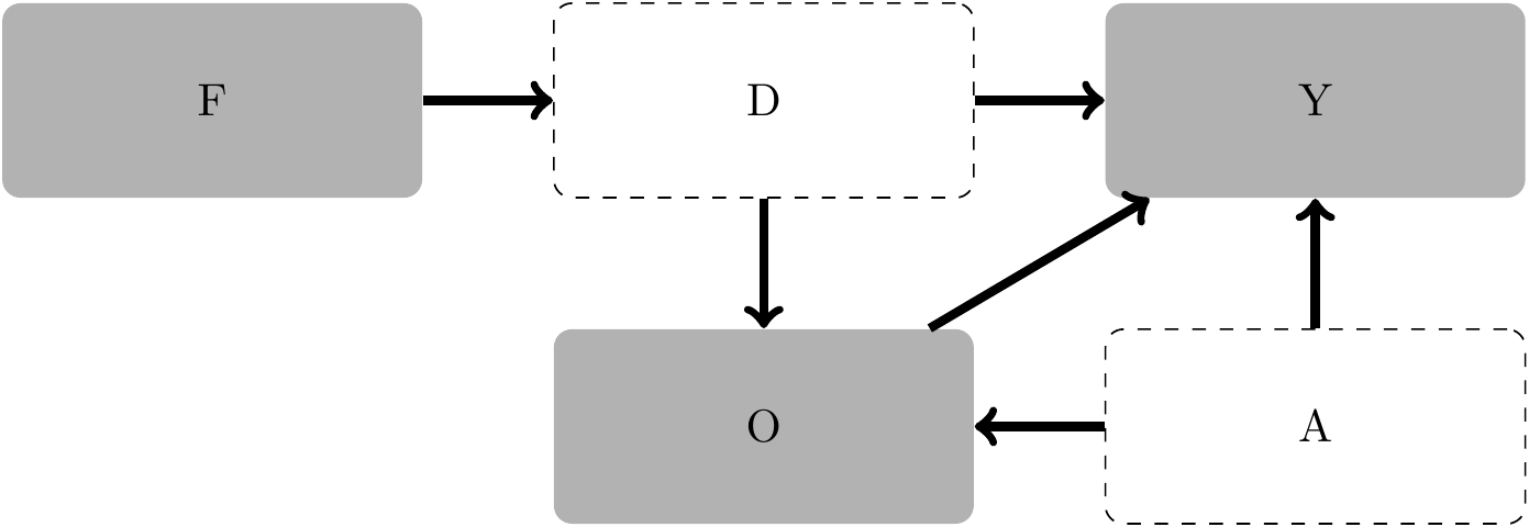
Note that there is in fact no effect of being female (\(F\)) on earnings (\(Y\)) except through discrimination (\(D\)). Thus, if we could control for discrimination, we’d get a coefficient of zero on \(F\). In this example, we aren’t interested in estimating the effect of being female on earnings per se; we are interested in estimating the effect of discrimination. Note also that discrimination is not directly observed, but given our DAG, we can use \(F\) as a proxy for \(D\), as we have assumed that there is no relation between \(F\) and \(Y\) (or between \(F\) and \(O\), which denotes occupational assignment) except through \(D\).
In this DAG, there are two paths between \(D\) and \(Y\):
\[ \begin{aligned} D &\rightarrow Y \\ D &\rightarrow O \rightarrow Y \end{aligned} \]
Neither path is a back-door path between \(D\) and \(Y\) because neither has an arrow pointing into \(D\). Conditioning on \(O\) causes the estimated effect of discrimination on income to be biased because \(O\) is a descendant of \(D\), and a set of conditioning variables \(Z\) satisfies the back-door criterion only if no node in \(Z\) is a descendant of \(D\).
To check our understanding of the application of the back-door criterion to this setting, we can generate some data based on a simulation that matches the causal diagram in Figure 4.5.
We run two regressions on these data and present results in Table 4.3.
| (1) | (2) | |
|---|---|---|
| (Intercept) | 3.013*** | 1.003*** |
| femaleTRUE | -5.005*** | -0.996*** |
| occupation | 1.999*** | |
| Num.Obs. | 100000 | 100000 |
| R2 | 0.556 | 0.911 |
4.4.1 Exercises
Given the equations for
occupationandsalaryin the simulation above, what is the direct effect of discrimination on salary? What is the indirect effect (i.e., the effect viaoccupation) of discrimination on salary? What is the total effect of discrimination on salary? How do each of these effects show up in the regression results reported in Table 4.3? (Note: Because of sampling variation, the relationships will not be exact.)-
Consider the possibility of an additional unobserved variable, ability (\(A\)), that affects role assignment (\(O\)) and also affects income (\(Y\)) directly. A DAG that captures this is provided in Figure 4.6.
What would be the correct conditioning strategy in this case? Would it now make sense to condition on \(O\) if the goal is to estimate the total effect of discrimination on \(Y\)? (Hint: In answering this question, it may help to adapt the simulation above to generate an
abilityvariable and to incorporate that in the model using code like the following.)
-
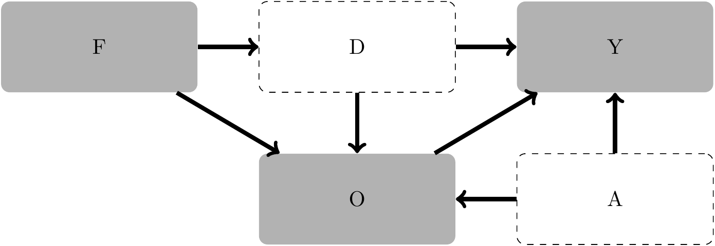
Consider the additional possibility of different occupational preferences between males and females, as depicted in Figure 4.7.
Given the DAG in Figure 4.7, is it possible to identify a set of conditioning variables that allow you to estimate the total effect of discrimination on salary? What roles does \(O\) have in this DAG? (Hint: Replace the
0coefficient onfemalein theoccupationequation used in the last question with a value of either-1or+1. Does the sign of this coefficient affect the sign of bias, if any?) Is it possible to estimate the direct effect of discrimination on salary? If so, how? If not, why?
4.5 Causal diagrams: Application in accounting
Many papers in accounting research include many variables to “control for” potential confounding effects. If these variables are truly confounders, then this is appropriate. However, Gow et al. (2016) suggest that researchers do not give consideration to the possibility that these variables are mediators or colliders. Inclusion of “controls” that are mediators or colliders will generally lead to bias, making it important to rule these possibilities out.
Larcker et al. (2007) discuss these distinctions, albeit in different language, in the context of corporate governance research and a regression model of the form:14
\[ Y = \alpha + \sum_{r=1}^R \gamma_r Z_r + \sum_{s=1}^S \beta_s X_s + \epsilon \tag{4.2}\]
Larcker et al. (2007) suggest that
“One important feature in the structure of Equation 4.2 is that the governance factors [\(X\)] are assumed to have no impact on the controls (and thus no indirect impact on the dependent variable). As a result, this structure may result in conservative estimates for the impact of governance on the dependent variable. Another approach is to only include governance factors as independent variables, or:
\[ Y = \alpha + \sum_{s =1}^S \beta_s X_s + \epsilon \tag{4.3}\]
The structure in Equation 4.3 would be appropriate if governance impacts the control variables and both the governance and control variables impact the dependent variable (i.e., the estimated regression coefficients for the governance variables will capture the total effect or the sum of the direct effect and the indirect effect through the controls).”
But Larcker et al. (2007) gloss over some subtle issues. If some elements of \(Z_r\) are mediators and other elements are confounders, then biased estimates will arise from both equations. The estimator based on Equation 4.3 will be biased because confounders have been omitted, while that based on Equation 4.2 will be biased because mediators have been included. Additionally, the claim that the estimates are “conservative” assumes that the indirect effect via mediators is of the same sign as the direct effect. Without this assumption, the relation between the direct effect and the total effect is unclear in both magnitude and even sign.
Additionally, Larcker et al. (2007) do not address possible colliders, which plausibly exist in their setting. For example, corporate governance plausibly affects firms’ choice of leverage, while performance also plausibly affects leverage. If so, “controlling for” leverage might induce associations between governance and performance even when there is no causal relation between these variables.15 While there is intuitive appeal to with-and-without-controls approach suggested by Larcker et al. (2007), selecting controls “requires careful thinking about the plausible causal relations between the treatment variables, the outcomes of interest, and the candidate control variables” (Gow et al., 2016, p. 485).
4.6 Further reading
Gow et al. (2016) covers several topics not covered in this chapter. But parts of this book (especially Part III) go into those topics more deeply than Gow et al. (2016) do.
More recent econometrics textbooks, such as Wooldridge (2010), more explicitly address causal inference than do older texts. In addition, a number of more recent textbooks—such as Angrist and Pischke (2008) and Cunningham (2021)—place causal inference front and centre.
Fuller coverage of causal diagrams can be found in Morgan and Winship (2014); Pearl (2009a) offers a more advanced treatment. Huntington-Klein (2021) uses causal diagrams as an organizing framework and spends much of the book examining causal inference before introducing the econometric tools that are the primary focus of most textbooks. A more accessible introduction to ideas in Pearl (2009a), including more recent developments, is provided by Pearl and Mackenzie (2019).
Our discussion of structural models glossed over some subtle, but important, issues that get some coverage in Chapter 5 of Pearl (2009a).
We provide some intuitive discussion of these ideas in Chapter 5.↩︎
You might find an entry on Granger causality, but with some caveat that this is a misnomer.↩︎
In contrast, the non-recognition of most internally generated intangible assets is not conditional on news, and it therefore considered unconditional conservatism.↩︎
The work of Ball et al. (2013) was in large part a response to results in Dietrich et al. (2007) that showed “bias” in the Basu (1997) measure. The careful reader might wonder how bias can arise if it is not clear what underlying parameter is being estimated. But Dietrich et al. (2007) choose their words carefully and merely seek to demonstrate bias in the test statistics in favour of a hypothesis of conservatism when none exists rather than bias in an estimate coefficient relative to its true value.↩︎
Dietrich et al. (2022) make some tentative steps in the direction of a model in which conservatism is parameterized by considering two different levels of conservatism in addition to the no-conservatism regime.↩︎
Here \(:=\) means “defined as …”.↩︎
Including variables in a linear regression framework is a form of parametric conditioning and “controls for” these variables only under strict assumptions, such as linearity in the relations between \(X\), \(Y\), and \(Z\).↩︎
Inclusion of \(Z\) blocks the “back-door” path from \(Y\) to \(X\) via \(Z\).↩︎
The quotes around the terms “direct effect” and “indirect effect” reflect that the meaning of these terms is very much contingent on what variables are included in the model.↩︎
The two arrows from \(X\) and \(Y\) “collide” in \(Z\).↩︎
The “arrow into \(X\)” is the portion of the definition that explains the “back-door” terminology.↩︎
How the quantities \(P(y|x)\) map into estimates of causal effects is not critical to the current discussion, it suffices to note that in a given setting, it can be calculated if the needed variables are observable.↩︎
This subsection is adapted from Cunningham (2021), available at https://mixtape.scunning.com.↩︎
We alter the mathematical notation and equation numbers of Larcker et al. (2007) to conform with notation and numbering we use here.↩︎
Note that Larcker et al. (2007) do not “control for” leverage in regressions where performance is a dependent variable.↩︎