13  Event studies

In previous chapters, we studied papers that have examined the reaction of financial markets to information. Chapter 10 covered Fama et al. (1969), which studied the adjustment of prices to the information in stock splits. Chapter 11 examined Ball and Brown (1968), which shows that market returns over a year are correlated with earnings news for the period. Chapter 12 studied Beaver (1968), which shows that volume and price volatility increase around earnings announcements.

The decades since those early papers have seen significant evolution in how researchers study the market reaction to information and this chapter provides an introduction to current event-study methods.

Tip

The code in this chapter uses the packages listed below. For instructions on how to set up your computer to use the code found in this book, see Section 1.2. Quarto templates for the exercises below are available at https://github.com/iangow/far_templates.

library(dplyr)
library(DBI)
library(ggplot2)
library(farr)
library(modelsummary)
library(dbplyr)        # window_order()

13.1 Overview

MacKinlay (1997, p. 13) defines an event study as one that, “using financial market data … measures the impact of a specific event on the value of a firm. The usefulness of such a study comes from the fact that, assuming highly efficient markets, the effects of an event will be reflected immediately in security prices.¹ Thus a measure of the event’s economic impact can be constructed using security prices observed over a relatively short time period.”

MacKinlay (1997, p. 14) continues: “In the late 1960s seminal studies by Ray Ball and Philip Brown (1968) and Eugene Fama et al. (1969) introduced the methodology that is essentially the same as that which is in use today. Ball and Brown considered the information content of earnings, and Fama et al. studied the effects of stock splits after removing the effects of simultaneous dividend increases.”

Event studies examine the impact of a class of identifiable events on one or more variables of economic interest. In capital markets research, the variable of economic interest is typically the returns of a firm’s shares around the event.

The basic ingredients of an event study are:

• A class of events: earnings announcements, merger announcements, stock splits, earnings forecast changes. In many research papers, these events represent the treatment of interest.
• An outcome variable of interest: accounting policy, market returns, trading volume.
• Control observations: observations for which the event did not occur.
• Control variables: additional variables that may be correlated with both the event—such as dividend announcements with earnings announcements or forecast revisions with earnings announcements—and also returns (see Chapter 4 for more on control variables).

Additionally, as we saw in Chapter 12, lining up observations in event time is a critical feature of most event studies.

13.1.1 Discussion questions

1. Does Ball and Brown (1968) meet the MacKinlay (1997) definition of an event study? What features are present and what, if any, are missing?

2. Does Beaver (1968) meet the MacKinlay (1997) definition of an event study? What features are present and what, if any, are missing?

13.2 The modern event study

The event study has evolved over time. While event studies today generally meet the definition in MacKinlay (1997), the event-study approach has changed as it has been adapted to a wider variety of situations.

One change is that researchers have become more interested in using event studies to understand the economic effects of regulation, rather than the market reaction to firm-specific announcements. Fama et al. (1969) studied stock-splits and Beaver (1968) studies earnings announcements. In each case, the events are firm-level events that are largely independent of each other (e.g., they are not excessively clustered in time). In contrast, each of the three more recent event studies we study below uses regulatory events such as events affecting the probability of legislation (Larcker et al., 2011; Zhang, 2007) or accounting standards going into effect (Khan et al., 2017).

A related change is an increased reliance on market efficiency, as the typical modern event study uses (in the words of MacKinlay, 1997) “security prices observed over a relatively short time period” as a “measure of the event’s economic impact”. Neither Fama et al. (1969) nor Beaver (1968) relies heavily on market efficiency in establishing that markets appear to react to stock-splits and earnings announcements, respectively, and neither study seeks to show whether stock split or earnings announcements create (or destroy) value. In contrast, the modern event study is often leaning on market efficiency to evaluate regulation. For example, using an event study to ask “do the FASB’s standards add shareholder value?” (Khan et al., 2017) relies heavily on the market having an informed view of the kind implied by stronger forms of market efficiency.

A consequence of this changed emphasis is that often there are fewer independent observations for the researcher to work with. For example, the primary analysis of Zhang (2007) focuses on four event windows, far fewer than the 506 earnings announcements in Beaver (1968). As we will see, researchers often use supplementary analyses to address the relative paucity of data.

13.2.1 A small event study

To better understand the modern event study, we conduct a mini-study of our own. Suppose that we want to understand better the value-creation process at Apple with a particular emphasis on Apple’s product development process. At the time of writing (mid-2022), Apple is the most valuable company in the world, with a market capitalization over US$2 trillion, so understanding how it creates value for shareholders may be of interest to researchers.

As Apple is notoriously secretive about its product pipeline, the media events at which its products are launched are closely watched affairs. For example, at the Macworld Conference & Expo San Francisco 2007 (9 January 2007), Apple announced the iPhone, which would go on to become Apple’s primary revenue source and one of the largest phone products in the world. At an Apple Special Event on 27 January 2010, Apple announced the iPad, Apple’s tablet computer.

So, to understand whether Apple’s products create value for Apple shareholders, we might run an event study using Apple’s media events as the events of interest.

The farr package includes the data frame apple_events, which is derived from data found on Wikipedia.² Let’s look at the last few rows of this table:

tail(apple_events)

# A tibble: 6 × 3
  event               event_date end_event_date
  <chr>               <date>     <date>        
1 Apple Special Event 2019-09-10 2019-09-10    
2 Apple Special Event 2019-12-02 2019-12-02    
3 WWDC 2020           2020-06-22 2020-06-26    
4 Apple Special Event 2020-09-15 2020-09-15    
5 Apple Special Event 2020-10-13 2020-10-13    
6 Apple Special Event 2020-11-10 2020-11-10    

We will need return data from CRSP to conduct our event study. We first need to get Apple’s PERMNO so we can look up returns on CRSP. Knowing that Apple’s ticker is AAPL helps.

PostgreSQL

db <- dbConnect(RPostgres::Postgres())

stocknames <- tbl(db, Id(schema = "crsp", table = "stocknames"))
dsf <- tbl(db, Id(schema = "crsp", table = "dsf"))
dsi <- tbl(db, Id(schema = "crsp", table = "dsi"))

idx_daily <- tbl(db, Id(schema = "comp", table = "idx_daily"))

parquet

db <- dbConnect(duckdb::duckdb())

stocknames <- load_parquet(db, schema = "crsp", table = "stocknames")
dsf <- load_parquet(db, schema = "crsp", table = "dsf")
dsi <- load_parquet(db, schema = "crsp", table = "dsi")

idx_daily <- load_parquet(db, schema = "comp", table = "idx_daily")

apple_permno <-
  stocknames |>
  filter(ticker == "AAPL") |>
  select(permno) |>
  distinct() |>
  pull()

apple_permno

[1] 14593

We then use Apple’s PERMNO (14593) to get return data from CRSP. In this case, we will get daily returns for Apple (ret) from crsp.dsf and value-weighted “market” returns (vwretd) from crsp.dsi and calculate market-adjusted returns as ret - vwretd.³ In this case, we will grab all returns since the start of 2005, which covers all the events on apple_events.

apple_rets <-
  dsf |>
  inner_join(dsi, by = "date") |>
  mutate(ret_mkt = ret - vwretd) |>
  select(permno, date, ret, ret_mkt, vol) |>
  filter(permno == apple_permno,
         date >= "2005-01-01") |>
  collect()

Unlike the earnings announcements that we studied in Chapter 12, Apple’s media events extend over multiple days, so our event windows also need to extend over multiple days. To allow for some leakage of information in the day before the start of the media events and to allow the market some time to process the value implications of the media event, we will set our event window from one trading day before the start of each media event through to one day after the end of the media event. We will use the get_event_dates() function from the farr package to this end; behind the scenes, this function uses the get_trading_dates() and get_annc_dates() functions to get tables like trading_dates and annc_dates, respectively, which we studied in Chapter 12.⁴

apple_event_dates <-
  apple_events |>
  mutate(permno = apple_permno) |>
  get_event_dates(db, 
                  end_event_date = "end_event_date",
                  win_start = -1, win_end = +1) 

tail(apple_event_dates)

# A tibble: 6 × 5
  permno event_date end_event_date start_date end_date  
   <int> <date>     <date>         <date>     <date>    
1  14593 2019-09-10 2019-09-10     2019-09-09 2019-09-11
2  14593 2019-12-02 2019-12-02     2019-11-29 2019-12-03
3  14593 2020-06-22 2020-06-26     2020-06-19 2020-06-29
4  14593 2020-09-15 2020-09-15     2020-09-14 2020-09-16
5  14593 2020-10-13 2020-10-13     2020-10-12 2020-10-14
6  14593 2020-11-10 2020-11-10     2020-11-09 2020-11-11

We now organize the data in a way that allows us to depict Apple’s returns graphically over time including information about media events.

apple_reg_data <-
  apple_rets |>
  left_join(apple_event_dates, 
            join_by(permno, date >= start_date, date <= end_date)) |>
  mutate(is_event = !is.na(start_date)) |>
  select(permno, date, ret, ret_mkt, vol, is_event)

Now we have the data we need, we can calculate cumulative returns using the cumprod() function and then plot these returns over time.⁵

apple_reg_data |>  
  arrange(date) |>
  mutate(cumret = cumprod(1 + coalesce(ret, 0)),
         switch = coalesce(is_event != lead(is_event), FALSE)) |>
  ggplot(aes(x = date, y = cumret)) +
  geom_line() +
  geom_ribbon(aes(ymax = if_else(!is_event | switch, cumret, NA),
                  ymin = 0, 
                  fill = "Non-event")) +
  geom_ribbon(aes(ymax = if_else(is_event | switch, cumret, NA),
                  ymin = 0, 
                  fill = "Event")) +
  theme(legend.position = "bottom")

Figure 13.1: Apple returns

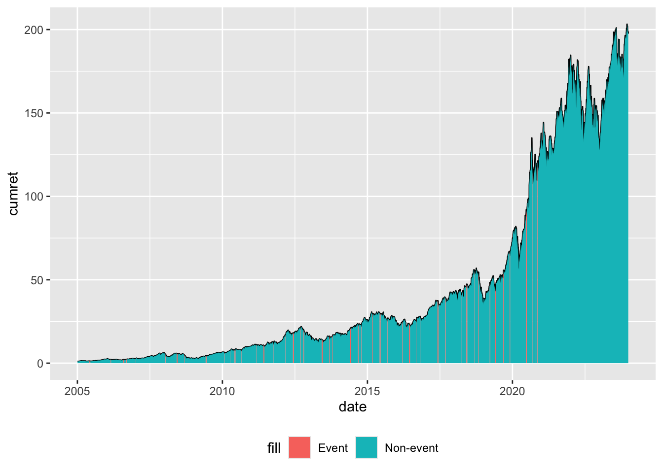
The line in Figure 13.1 represents cumulative returns since the start of the window. Two “area” plots are added to this line: one for the non-event windows and one for the event windows. The vast majority of dates are non-event dates, which makes the event windows difficult to discern in the plot. But “zooming in” makes the event windows easier to discern, as seen in Figure 13.2, which focuses on the last quarter of 2020.

apple_reg_data |>  
  arrange(date) |>
  mutate(cumret = cumprod(1 + coalesce(ret, 0)),
         switch = coalesce(is_event != lead(is_event), FALSE)) |>
  filter(date >= "2020-09-01", date <= "2020-12-31") |>
  ggplot(aes(x = date, y = cumret)) +
  geom_line() +
  geom_ribbon(aes(ymax = if_else(!is_event | switch, cumret, NA),
                  ymin = 0, fill = "Non-event")) +
  geom_ribbon(aes(ymax = if_else(is_event | switch, cumret, NA),
                  ymin = 0, fill = "Event")) +
  theme(legend.position = "bottom")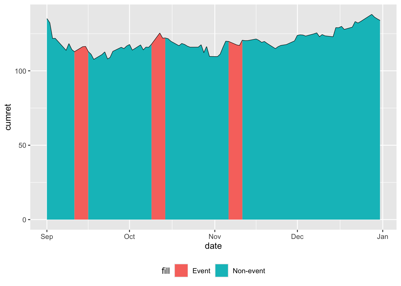

Figure 13.2: Apple returns: “Zoomed in”

There is little in the plots above to suggest that Apple media events are associated with unusual returns, but we will use regression analysis to test this more formally. We consider whether returns are different when the indicator variable is_event is TRUE. Inspired by Beaver (1968) (Chapter 12), we also consider the absolute value of returns (similar to squared return residuals used in Beaver (1968)) and relative trading volume.

fms <- list("ret_mkt" = lm(ret_mkt ~ is_event, data = apple_reg_data),
            "abs(ret)" = lm(abs(ret) ~ is_event, data = apple_reg_data),
            "Volume" = lm(vol/mean(vol) ~ is_event, data = apple_reg_data))

modelsummary(fms,
             estimate = "{estimate}{stars}",
             statistic = NULL,
             gof_map = c("nobs", "r.squared"),
             stars = c('*' = .1, '**' = 0.05, '***' = .01))

Table 13.1: Regression analysis of Apple media events

	ret_mkt	abs(ret)	Volume
(Intercept)	0.001***	0.014***	0.997***
is_eventTRUE	−0.002**	0.001	0.060
Num.Obs.	4781	4781	4781
R2	0.001	0.000	0.000

These regression analyses—interpreted fairly casually—provide evidence of lower returns, but not higher (or lower) levels of either trading volume or return volatility.

The code above examines whether returns for Apple during event periods behave differently from returns during non-event periods. Another function from farr, get_event_cum_rets(), calculates cumulative raw returns and cumulative abnormal returns using two approaches: market-adjusted returns and size-adjusted returns over event windows. Here we use this function to get cumulative returns over the windows around each Apple event.

rets <-
  apple_events |>
  mutate(permno = apple_permno) |> 
  get_event_cum_rets(db,
                     win_start = -1, win_end = +1,
                     end_event_date = "end_event_date")

We first look at market-adjusted returns, which on average barely differ from zero.

summary(rets$ret_mkt)

     Min.   1st Qu.    Median      Mean   3rd Qu.      Max. 
-0.103895 -0.026442 -0.007217 -0.005840  0.014285  0.135833 

We then ask: How many media events are positive-return events?

summary(rets$ret_mkt > 0)

   Mode   FALSE    TRUE 
logical      26      21 

(Answer: Fewer than half!)

Finally, we produce a scatter plot of market-adjusted returns for Apple media events by event date (Figure 13.3).

rets |>
  ggplot(aes(x = event_date, y = ret_mkt)) +
  geom_point() +
  geom_smooth(method = "lm", formula = "y ~ 1")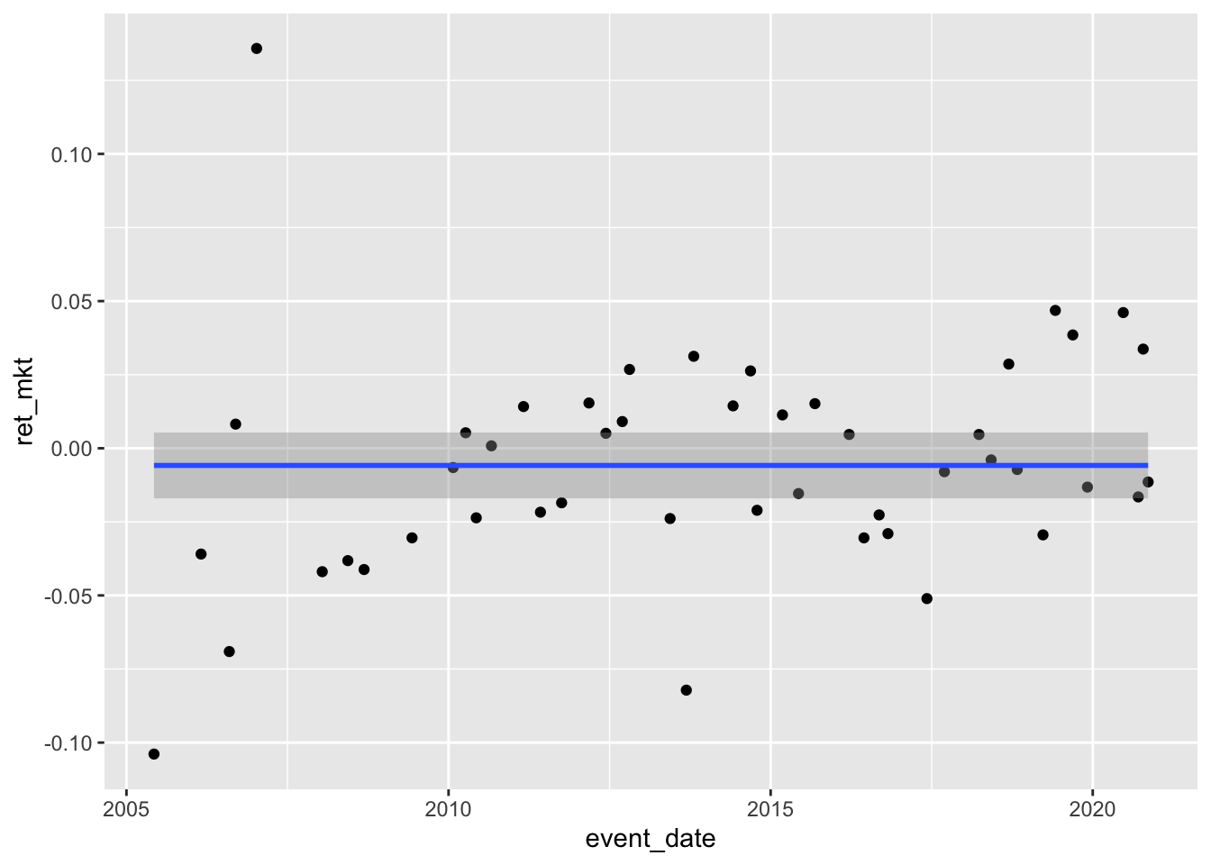

Figure 13.3: Apple market-adjusted returns and media events

13.2.2 Exercises

1. How would you expect the plot to change if we used cumret = exp(cumsum(log(1 + coalesce(ret, 0)))) in place of cumret = cumprod(1 + coalesce(ret, 0)) in creating the plot above? Is there any reason to prefer one calculation over time other?

2. Do we get different results in this case if we use cumret = cumprod(1 + ret) (i.e., remove the coalesce() function)? If so, why? If not, would we always expect this to be case (e.g., for stocks other than Apple)?

13.3 Event studies and regulation

Zhang (2007, p. 74) “investigates the economic consequences of the Sarbanes–Oxley Act (SOX) by examining market reactions to related legislative events.” Zhang (2007, p. 75) finds that “the cumulative value-weighted (equal-weighted) raw return of the U.S. market amounts to –15.35% (–12.53%) around the key SOX events.” As Zhang (2007) uses CRSP returns for the US market, we collect a local copy of the relevant data.

dsi_local <-
  dsi |>
  select(date, vwretd, ewretd) |>
  collect()

Zhang (2007, p. 76) focuses some analyses on “key SOX events” (defined below) and finds that “the estimated U.S. cumulative abnormal returns range from –3.76% and –8.21% under alternative specifications and are all statistically significant.” Here “all” means for each of value-weighted and equal-weighted returns and using abnormal returns relative to each of two models. For convenience, we focus on the model that measures abnormal returns relative as returns not explained by a “market model” where the market comprises Canadian stocks not listed in the US and omit analysis of the second model, which blends returns on several non-US portfolios as a benchmark. To this end, we collect data on returns for the Toronto composite index (gvkeyx == "000193") from Compustat’s index data (comp.idx_daily) over 2001 and 2002 and merge this data set with our local copy of crsp.dsi.

can_rets <-
  idx_daily |> 
  filter(gvkeyx == "000193") |> 
  window_order(datadate) |>
  mutate(ret_can = if_else(lag(prccd) > 0, prccd/lag(prccd) - 1, NA)) |> 
  filter(datadate >= "2000-01-01", datadate <= "2002-12-31") |>
  rename(date = datadate) |>
  select(date, ret_can) |>
  collect()

We collect data on 100 days of returns prior to 2001-12-28 because the analyses in Zhang (2007, p. 88) are “estimated using daily return data in the 100 days prior to December 28, 2001.”

reg_data <-
  dsi_local |>
  inner_join(can_rets, by = "date") |>
  filter(date < "2001-12-28") |>
  top_n(100, wt = date) 

We then fit models for market returns for both equal-weighted and value-weighted portfolios against Canadian returns.

fm_vw <- lm(vwretd ~ ret_can, data = reg_data)
fm_ew <- lm(ewretd ~ ret_can, data = reg_data)

We then use these models to calculate excess returns for all observations. In the following code we use pick(everything()), which is an idiom that we use in a few places in this book. In the function following the native pipe (|>), we often access the data frame supplied by the item preceding |> using the pipe placeholder _. However, this placeholder is not accessible to functions inside mutate(). Fortunately, we can use pick() instead. The pick() function provides a way to easily select columns from data inside a function like mutate(). In the current setting we can use everything() to indicate that we want to select all variables in the source data. As such, pick(everything()) is a handy workaround to the limitations of the pipe placeholder _.

dsi_merged <-
  dsi_local |>
  inner_join(can_rets, by = "date") |>
  mutate(abret_vw = vwretd - predict(fm_vw, pick(everything())),
         abret_ew = ewretd - predict(fm_ew, pick(everything()))) |>
  select(-ret_can)

From Table 2, Zhang (2007) appears to calculate the daily standard deviation of returns at about 1.2%. The exact basis for this calculation is unclear, but similar analyses are “estimated using daily return data in the 100 days prior to December 28, 2001” (Zhang, 2007, p. 88), so we calculate the daily volatility on this basis using the following calculation, which yields the value 1.28%

sd_ret <-
  dsi_local |>
  filter(date < "2001-12-28") |>
  top_n(100, wt = date) |>
  summarize(sd(vwretd)) |>
  pull()

The farr package contains the data frame zhang_2007_windows containing the dates of the event windows found in Table 2 of Zhang (2007). We can combine these data with return data from dsi_local to calculate cumulative returns for each event window. Following Zhang (2007), we can estimate the standard error by scaling the daily return volatility by the square-root of the number of trading days in each window to calculate a \(t\)-statistic for each event. We use the standard deviation of residuals to estimate the daily volatility of the abnormal-return models.

zhang_2007_rets <-
  zhang_2007_windows |>
  inner_join(dsi_merged, join_by(beg_date <= date, end_date >= date)) |>
  group_by(event) |>
  summarize(n_days = n(),
            vwret = sum(vwretd),
            ewret = sum(ewretd),
            abret_vw = sum(abret_vw),
            abret_ew = sum(abret_ew),
            vw_t = vwret / (sqrt(n_days) * sd_ret),
            ew_t = ewret / (sqrt(n_days) * sd_ret),
            abret_vw_t = abret_vw / (sqrt(n_days) * sd(fm_vw$residuals)),
            abret_ew_t = abret_ew / (sqrt(n_days) * sd(fm_ew$residuals)))

In subsequent analyses, Zhang (2007) focuses on “key SOX events”, which seem to be those events with a “statistically significant” return at the 10% level in a two-tailed test, and reports results in Panel D of Table 1 (2007, pp. 91–92). We replicate the key elements of this procedure and our results correspond roughly with those reported in Zhang (2007) as “CAR2”.

zhang_2007_res <-
  zhang_2007_rets |>
  filter(abs(vw_t) > abs(qnorm(.05))) |>
  summarize(vwret = sum(vwret),
            ewret = sum(ewret),
            abret_vw = sum(abret_vw),
            abret_ew = sum(abret_ew),
            n_days = sum(n_days),
            vw_t = vwret / (sqrt(n_days) * sd_ret),
            ew_t = ewret / (sqrt(n_days) * sd_ret),
            abret_vw_t = abret_vw / (sqrt(n_days) * sd(fm_vw$residuals)),
            abret_ew_t = abret_ew / (sqrt(n_days) * sd(fm_ew$residuals)))

dbDisconnect(db)

We estimate cumulative raw value-weighted returns for the four “key SOX events” at \(-15.2\%\) (\(t\)-statistic \(-3.18\)), quite close to the value reported in Zhang (2007) (\(-15.35\%\) with a \(t\)-statistic of \(-3.49\)). However, our estimate of cumulative abnormal value-weighted returns for the four “key SOX events” is \(-3.18\%\) (\(t\)-statistic \(-1.02\)), which is closer to zero than the value reported in Zhang (2007) (\(-8.21\%\) with a \(t\)-statistic of \(-2.99\)), which is the only value of eight reported in Panel D of Table 1 that is statistically significant at conventional levels (5% in two-tailed tests).

13.3.1 Discussion questions

13.3.1.1 Zhang (2007)

1. What are the relative merits of raw and abnormal returns in evaluating the effect of SOX on market values of US firms? What do you observe in the raw returns for Canada, Europe, and Asia for the four events that are the focus of Panel B of Table 2 of Zhang (2007)? Does this raise concerns about Zhang (2007)’s results?

2. Describe the process for constructing the test statistics reported in Panel D of Table 2. How compelling are these results? Do you agree with the assessment by Leuz (2007, p. 150) that Zhang (2007) is “very careful in assessing the significance of the event returns”?

3. Describe in detail how you might conduct statistical inference using randomization inference in the setting of Zhang (2007) (see Section 19.7 for more on this approach)? What are the challenges faced and design choices you need to make in applying this approach? Does your approach differ from the bootstrapping approach used in Zhang (2007)?

4. Leuz (2007) identifies studies other than Zhang (2007) that find evidence that SOX was beneficial to firms? How can these sets of results be reconciled? What steps would you look to undertake to evaluate the conflicting claims of the two papers?

13.3.1.2 Khan et al. (2017)

1. What is the research question examined in Khan et al. (2017)? (Hint: Read the title.)

2. Khan et al. (2017, p. 210) argue that “an ideal research design to evaluate the benefits of accounting standards is to compare a voluntary disclosure regime, in which firms disclose information required by a particular standard, with a mandatory disclosure regime, in which firms are required to disclose that same information.” Do you agree that this research design would be “ideal” to address the question? What is the implied treatment in this ideal design?

3. Compare the Apple event study above with Khan et al. (2017). What are the relative strengths and weaknesses of the two studies? Do you think an event-study approach is appropriate for addressing the question “do Apple products add value?” Do you think an event-study approach is appropriate for addressing the research question of Khan et al. (2017)? Why or why not?

4. Do you think that standard-setters would view “reduction in estimation risk” as a goal of accounting standards? Evaluate the quality of the arguments linking improved standards to reduced estimation risk. The null hypothesis for Panel A is that the CAR of affected firms is not different from CAR of unaffected firms. How appropriate is it to report “most negative” and “most positive” CAR differences only? (Hint: If the null hypothesis is true, how many standards might you expect to have “statistically significant” coefficients?)

5. Interpret the results of Table 5, Panel B of Khan et al. (2017).

13.3.1.3 Larcker et al. (2011) “LOT”

1. How do LOT and FFJR differ in terms of the role of market efficiency in their research designs?

2. Consider Table 1 of LOT. What are the differences between the event study design in LOT from that in FFJR? What are implications of these differences?

3. How do you think Table 1 was developed? Do you see potential problems in the process underlying Table 1? Can you suggest alternative approaches to developing Table 1?

4. Consider proxy access, as some of the core results of the paper relate to proxy access. If you were a shareholder in a company, what concerns might you have about proxy access? Why might this decrease the value of your shares? Think about this is concrete terms; be specific about the kinds of circumstances where value will be reduced. How well do the variables NLargeBlock and NSmallCoalitions measure the exposure of firms to the issues you identified in the previous question? (As part of this, consider the timing of variable measurement relative to the timing of possible value-reducing outcomes.)

5. LOT makes use of a number of Monte Carlo simulations. How do these compare with the bootstrapping analyses conducted by Zhang (2007)? Are the simulations addressing the same underlying issues as Zhang (2007) bootstrapping approach?

Ball, R., Brown, P., 1968. An empirical evaluation of accounting income numbers. Journal of Accounting Research 6, 159–178. https://doi.org/10.2307/2490232

Beaver, W.H., 1968. The information content of annual earnings announcements. Journal of Accounting Research 6, 67–92. https://doi.org/10.2307/2490070

Fama, E.F., Fisher, L., Jensen, M.C., Roll, R., 1969. The adjustment of stock prices to new information. International Economic Review 10, 1–21. https://doi.org/10.2307/2525569

Khan, U., Li, B., Rajgopal, S., Venkatachalam, M., 2017. Do the FASB’s standards add shareholder value? The Accounting Review 93. https://doi.org/10.2308/accr-51840

Larcker, D.F., Ormazabal, G., Taylor, D.J., 2011. The market reaction to corporate governance regulation. Journal of Financial Economics 101, 431–448. https://doi.org/10.1016/j.jfineco.2011.03.002

Leuz, C., 2007. Was the Sarbanes–Oxley Act of 2002 really this costly? A discussion of evidence from event returns and going-private decisions. Journal of Accounting and Economics 44, 146–165. https://doi.org/10.1016/j.jacceco.2007.06.001

MacKinlay, A.C., 1997. Event studies in economics and finance. Journal of Economic Literature 35, 13–39.

Zhang, I.X., 2007. Economic consequences of the Sarbanes-Oxley Act of 2002. Journal of Accounting and Economics 44, 74–115. https://doi.org/10.1016/j.jacceco.2007.02.002

---

1. In terms of the discussion in Section 10.1, the required notion of market efficiency here is the ”price is right” notion.

2. See here for information on these events.

3. MacKinlay (1997, p. 18) points out that “the market-adjusted return model can be viewed as a restricted market model with \(\alpha_i\) constrained to be zero and \(\beta_i\) constrained to be one.”

4. For more on get_event_dates, type ? get_event_dates in the console of RStudio.

5. The purpose of the variable switch is to “fill” gaps in the plot that would arise in its absence. To see what this variable is doing, replace switch = coalesce(is_event != lead(is_event), FALSE) with switch = FALSE. These gaps are more apparent in Figure 13.2 than they are in Figure 13.1.