25  Matching

In Chapter 4, we discussed three basic causal diagrams and suggested that the concept of nonparametric conditioning on \(Z\) is more demanding than simply including \(Z\) as another regressor in a linear regression model. This chapter develops this idea more fully and examines practical approaches to properly conditioning on confounding variables.

Tip

The code in this chapter uses the following packages. We load tidyverse because we use several packages from the Tidyverse. For instructions on how to set up your computer to use the code found in this book, see Section 1.2. Quarto templates for the exercises below are available at https://github.com/iangow/far_templates.

library(tidyverse)
library(DBI)
library(farr)
library(dbplyr)        # window_order()
library(fixest)
library(modelsummary)
library(MatchIt)       # match.data(), matchit()

25.1 Background on auditor choice

For concreteness, we will explore the basic ideas of this chapter using the setting of auditor choice and its effects. An extensive literature has examined the question of whether “Big N” auditors produce higher audit quality. This question is examined in two of the papers we will study in this chapter (DeFond et al., 2017; Lawrence et al., 2011).

For data on auditors, the table comp.funda has a column labelled au , which lines up with aucd in comp.r_auditors.

PostgreSQL

db <- dbConnect(RPostgres::Postgres(), bigint = "integer")

company <- tbl(db, Id(schema = "comp", table = "company"))
funda <- tbl(db, Id(schema = "comp", table = "funda"))
r_auditors <- tbl(db, Id(schema = "comp", table = "r_auditors"))

parquet

db <- dbConnect(duckdb::duckdb())

company <- load_parquet(db, schema = "comp", table = "company")
funda <- load_parquet(db, schema = "comp", table = "funda")
r_auditors <- load_parquet(db, schema = "comp", table = "r_auditors")

While Lawrence et al. (2011) refers to the “Big Four”, they are actually referring to the current group that DeFond et al. (2017) refer to as the “Big N”. The latter term alludes to the prior incarnations of the set of top audit firms, including the “Big Five” (prior to the demise of Arthur Andersen” and the “Big Eight” (prior to mergers in the late 1980s) (see Gow and Kells, 2018 for more on this history).

r_auditors |> arrange(aucd) |> collect(n = 12)

Table 25.1: Values of aucd for top auditors

aucd	audesc
0	Unaudited
1	Arthur Andersen
2	Arthur Young
3	Coopers & Lybrand
4	Ernst & Young
5	Deloitte & Touche
6	KPMG Peat Marwick
7	PricewaterhouseCoopers
8	Touche Ross
9	Other
10	Altschuler, Melvoin, and Glasser
11	BDO Seidman

Looking closer at r_auditors, we see that Arthur Andersen has an aucd of 1. Note that Arthur Young is now part of Ernst & Young, Coopers & Lybrand is now part of PricewaterhouseCoopers, and Touche Ross is now part of Deloitte & Touche. So a reasonable approach to “Big N” would appear to be big4 = aucd %in% 1:8L.¹ It’s commonly understood that most large firms choose a Big Four auditor. But rather than simply accepting that, we can look at the data.

Here we focus on firms with meaningful financial statements (sale > 0, at > 0) and fiscal 2019, the latest fiscal year with complete data at the time of first writing this chapter.

size_big4 <-
  funda |>
  filter(indfmt == "INDL", datafmt == "STD",
         consol == "C", popsrc == "D") |>
  filter(sale > 0, at > 0, fyear == 2019, !is.na(au)) |>
  mutate(au = as.integer(au)) |>
  select(gvkey, datadate, fyear, au, prcc_f, csho) |>
  mutate(big4 = au %in% 1:8L,
         mkt_cap = prcc_f * csho * 1e6) |>
  arrange(gvkey, datadate) |>
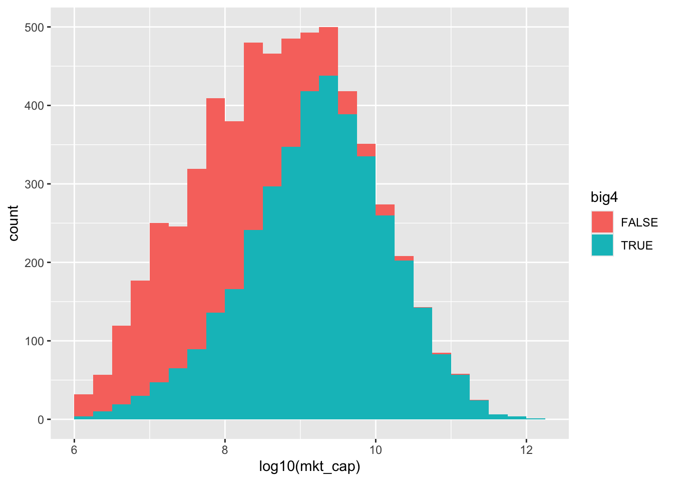
  collect()

We calculate market share by “bins” where each bin represents an order of magnitude of market capitalization. For example, (9, 10] includes all firms with market capitalization over $1 billion (\(10^9\)) and less than or equal to $10 billion (\(10^{10}\)).

size_big4 |> 
  filter(mkt_cap > 1e6) |> 
  mutate(log_mkt_cap = log10(mkt_cap)) |>
  mutate(bin = cut(log_mkt_cap, breaks = seq(6, 13, 1))) |>
  group_by(bin) |>
  summarize(big4_perc = 100 * mean(big4),
            big4_num = sum(big4),
            non_big4_num = sum(!big4))

Table 25.2: Big 4 market share by market capitalization

bin	big4_perc	big4_num	non_big4_num
(6,7]	16.36364	63	322
(7,8]	27.55519	337	886
(8,9]	58.03424	1051	760
(9,10]	89.67083	1580	182
(10,11]	96.76056	687	23
(11,12]	97.84946	91	2
(12,13]	100.00000	1	0

Interestingly, one of the two cases of companies with an apparent market capitalization over $100 billion (\(10^{11}\)) and a non–Big Four auditor is Vanjia, which apparently misstated the number of its shares outstanding as 8,550 million rather than 30 million.²

size_big4 |>
  filter(!big4, mkt_cap > 1e11) |>
  mutate(fyear = as.character(fyear))

Table 25.3: Two large non-Big 4 firms

gvkey	datadate	fyear	au	prcc_f	csho	big4	mkt_cap
014447	2019-12-31	2019	9	92.988	2,518.262	FALSE	234,168,146,856
026478	2019-12-31	2019	9	14.380	8,550.000	FALSE	122,949,000,000

We can also present the data as a histogram. From either Table 25.2 or Figure 25.1, it is clear that the Big Four have overwhelming market share among the largest firms and have most of the market even among firms with market capitalization in the $100 million-to-$1 billion range.

size_big4 |> 
  filter(mkt_cap > 1e6) |> 
  ggplot(aes(x = log10(mkt_cap), fill = big4)) +
  geom_histogram(breaks = seq(6, 12.25, 0.25))

Figure 25.1: Histogram of market capitalization with auditor type

25.2 Simulation analysis

One challenge for an empirical researcher studying the effect of having a Big Four auditor is that market capitalization is plausibly a confounding variable, or confounder, of the kind seen in Figure 4.1. That is, having a large market capitalization is likely to cause—or be associated with variables that cause—firms to choose a Big Four auditor and also to affect a variety of economic outcomes that may be of interest, such as accounting quality. We know from our analysis in Chapter 4 that we want to “control for” confounders but we show here that this is not always as simple as including the confounding variable in OLS regression.

In this section, we use simulation analysis to examine more closely how to control for confounding variables. We start with the actual empirical distribution of market capitalization from the data depicted in the histogram above. For each bin in the histogram depicted in Figure 25.1, we calculate the observed conditional probability of a firm in that bin having a Big Four auditor and store the results in prob_big4.

prob_big4 <-
  size_big4 |>
  filter(mkt_cap > 1e6) |> 
  select(big4, mkt_cap) |>
  mutate(log_mkt_cap = log10(mkt_cap)) |>
  mutate(bin = cut(log_mkt_cap, breaks = seq(6, 12.25, 0.25))) |>
  group_by(bin) |>
  mutate(p_big4 = mean(big4)) |>
  ungroup()

We then run our simulation. We draw 5000 firms from this distribution and assign each firm an auditor based on the conditional probabilities calculated above. A critical assumption here is that, conditional on market capitalization, whether a Big Four auditor is chosen is completely random. Finally, we calculate a measure of audit quality that is a non-linear function of market capitalization and a random noise component. We explain the role of pick(everything()) in Chapter 13.

n_firms <- 5000

set.seed(2021)
sim_auditor <-
  prob_big4 |>
  sample_n(size = n_firms) |>
  mutate(rand = runif(nrow(pick(everything()))),
         big4 = rand < p_big4,
         epsilon = rnorm(nrow(pick(everything()))),
         id = 1:nrow(pick(everything()))) |>
  mutate(audit_quality = big4 * 0 + mkt_cap^(1/3) * 0.003 + epsilon) |>
  select(id, big4, mkt_cap, log_mkt_cap, audit_quality)

Given this is a simulation, we know that the correct causal diagram is that shown in Figure 25.2.

Figure 25.2: Market capitalization is a confounder

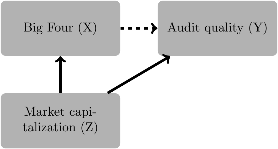
We draw the arrow connecting \(X\) and \(Y\) with a dashed line because the true coefficient on big4 is zero, so in this simulation there is no actual causal relation between big4 and audit_quality. Of course, in reality, we would not know this fact and would need to infer it from data.

The good news from this causal diagram is that correctly conditioning on \(Z\) should give us an unbiased estimator of the causal effect of \(X\) on \(Y\). So let’s regress audit_quality on big4 and mkt_cap.

fm <- lm(audit_quality ~ big4 + I(mkt_cap / 1e9), 
         data = sim_auditor)         
modelsummary(fm,
             estimate = "{estimate}{stars}",
             gof_map = c("nobs", "r.squared"),
             stars = c('*' = .1, '**' = 0.05, '***' = .01))

Table 25.4: Regression of audit quality using simulated data

	(1)
(Intercept)	1.561***
	(0.050)
big4TRUE	2.310***
	(0.064)
I(mkt_cap/1e+09)	0.057***
	(0.001)
Num.Obs.	5000
R2	0.555

In Table 25.4 we see a clearly positive coefficient on big4 even though we are “controlling for” mkt_cap, and we might be tempted to conclude that we have identified a causal effect. Of course, we know that this conclusion is invalid. The issue is that we are effectively assuming a linear relation between mkt_cap and audit quality, whereas the true relation is non-linear in mkt_cap. As a result, “controlling for” mkt_cap by including mkt_cap in a regression does not adequately control for the relation between mkt_cap and audit quality. Because there is a non-linear relation between big4 and mkt_cap, the regression specification can use information in big4 to explain variation in audit_quality in addition to that variation explained by a linear function of mkt_cap. This additional explanatory power shows up as a statistically significant coefficient on big4 in the regression above.

Would some kind of matching analysis help?

Given its prominence in accounting research, we will focus on propensity-score matching here. In this section, we present propensity-score matching as a recipe of sorts. We then evaluate how well it does in our simulated settings before discussing some aspects of the theory for why we might expect it to work.

The first step in our recipe is the estimation of propensity scores, which are estimates of the probability of receiving treatment as a function of observed variables. The most common approach is to use logistic regression, which we can do using glm(), as seen in Chapter 23.

sim_fm <- glm(!big4 ~ mkt_cap, data = sim_auditor, 
              family = binomial(link = "logit"))

We can estimate propensity scores as the fitted values from the estimated logit model (we specify type = "response" to get fitted values on the original \([0, 1]\) scale of the dependent variable).

sim_match_pscores <-
  sim_auditor |>
  mutate(pscore = predict(sim_fm, type = "response"))

The second step in the recipe is to matching treatment observations to their nearest counterparts among the control observations, where “nearest” means closest in terms of propensity scores. But even with the propensity score, we need an algorithm To this end, we can use matchit() function the MatchIt package. This function returns a matchit object to which we can apply match.data() to retrieve the resulting matches, which we store in sim_matches. Following Lawrence et al. (2011), we use a caliper of 3% use !big4 as the dependent variable, as not having a Big Four auditor is the less common condition.

sim_matches <- 
  matchit(!big4 ~ mkt_cap, data = sim_match_pscores, caliper = 0.03) |>
  match.data()

Inspecting sim_matches, we see that it contains the variable distance that exactly matches pscore that we estimated above.

sim_matches |> count(pscore == distance)

# A tibble: 1 × 2
  `pscore == distance`     n
  <lgl>                <int>
1 TRUE                  2388

In addition to the original contents of sim_auditor for the matched observations, sim_matches contains data on the matched pairs in the column subclass. Picking observations for three arbitrary values of subclass, we can see that each value is associated with a pair of observations, one with big4 == FALSE and one with big4 == TRUE and very similar values of mkt_cap and hence very similar pscore values.

sim_matches |> 
  filter(subclass %in% c(220, 481, 333)) |> 
  select(id, big4, mkt_cap, pscore, subclass) |>
  arrange(subclass, big4)

Table 25.5: Sample matched pairs

id	big4	mkt_cap	pscore	subclass
179	FALSE	197,311,500	0.513	220
2,287	TRUE	258,819,200	0.508	220
2,237	FALSE	3,172,390	0.531	333
2,165	TRUE	10,452,750	0.530	333
2,784	FALSE	30,094,100	0.528	481
2,034	TRUE	93,405,180	0.523	481

To examine the success of the match, we can compare two pairs of histograms. The first pair Figure 25.3 shows the propensity scores for all observations. Here we see that there are many treatment observations with p-scores above say 0.70, but very few control observations with comparable p-scores to match with these. In this relatively simple setting, this is really just another way of saying there are many large Big Four clients and few similarly sized non–Big Four clients to match with them. This suggests that many observations will be unmatched.

The first pair of histograms Figure 25.4 shows the propensity scores for the matched observations. We can see that the distributions of p-scores for treatment and control observations look very similar, suggesting a fairly good match.

sim_match_pscores |> 
  ggplot(aes(x = pscore, fill = big4)) + 
  geom_histogram(binwidth = 0.025) + 
  facet_grid(big4 ~ .) +
  theme(legend.position = "none")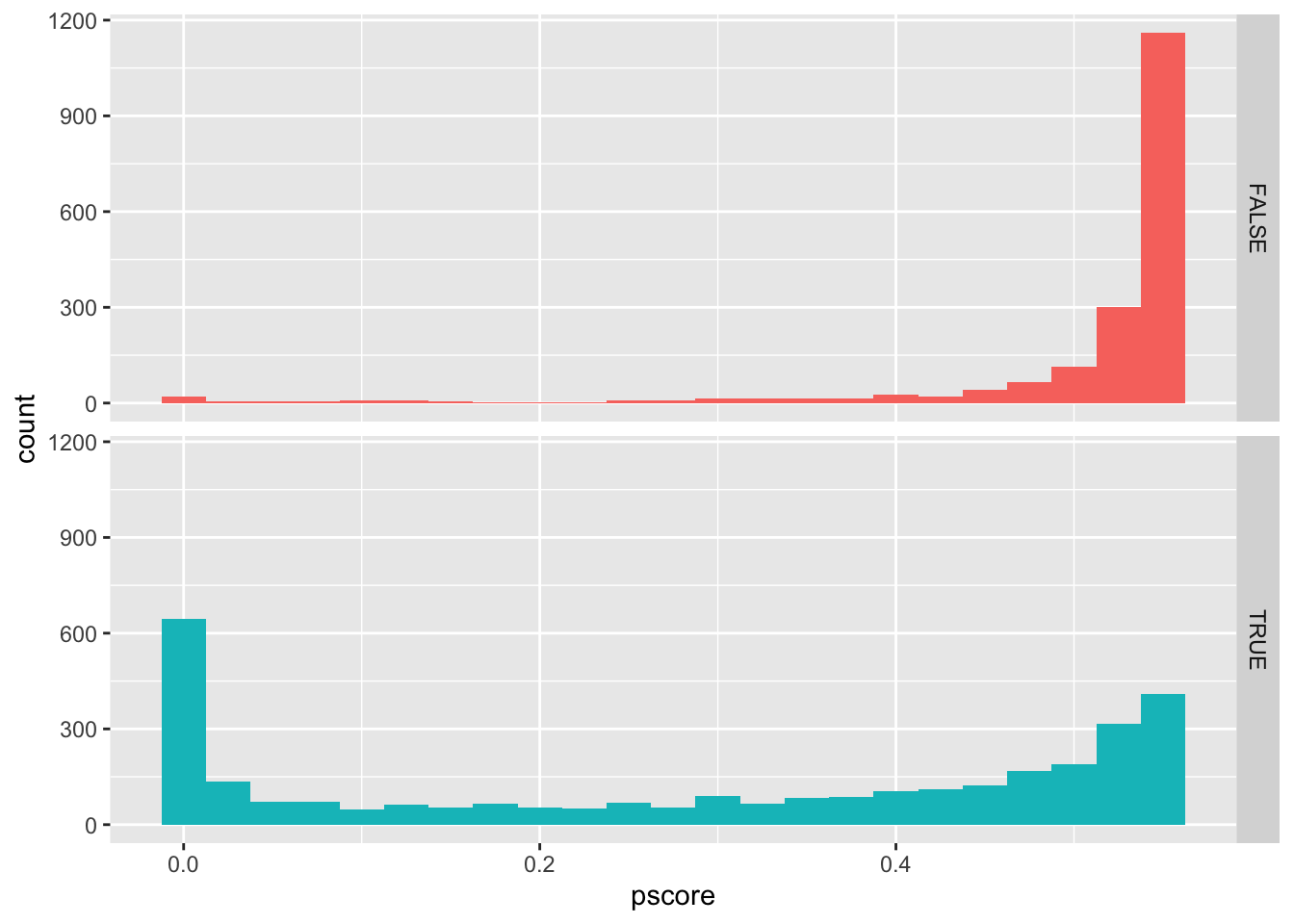

Figure 25.3: Propensity scores distribution: All observations

sim_matches |> 
  ggplot(aes(x = pscore, fill = big4)) + 
  geom_histogram(binwidth = 0.025) + 
  facet_grid(big4 ~ .) +
  theme(legend.position = "none")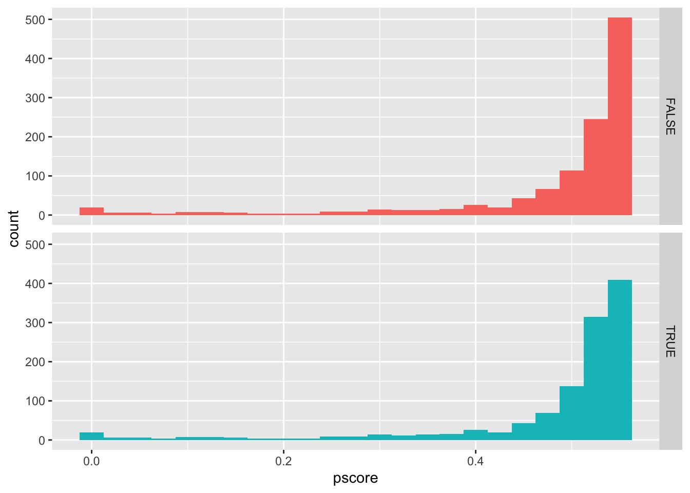

Figure 25.4: Propensity scores distribution: Matched observations

If we are happy with the match, we can finish our analysis by estimating regressions. Like Lawrence et al. (2011), we estimate regressions with and without the variables from the p-score regression (Shipman et al., 2016 refer to these approaches as “MR” and “t-test,” respectively).

fms <- list(feols(audit_quality ~ big4, data = sim_matches),
            feols(audit_quality ~ big4 + I(mkt_cap / 1e9), 
                  data = sim_matches))

modelsummary(fms,
             estimate = "{estimate}{stars}",
             gof_map = c("nobs", "r.squared"),
             stars = c('*' = .1, '**' = 0.05, '***' = .01))

Table 25.6: Relation between big4 and audit quality (matched)

	(1)	(2)
(Intercept)	1.893***	1.755***
	(0.050)	(0.044)
big4TRUE	0.234***	0.241***
	(0.071)	(0.061)
I(mkt_cap/1e+09)		0.129***
		(0.005)
Num.Obs.	2388	2388
R2	0.005	0.259

Interestingly, we see that big4 still has a statistically significant relation with audit quality. This is likely due to a residual effect of mkt_cap being picked up by big4 due to the imperfection of the propensity-score match.

25.2.1 Exercises

1. What happens in the above analyses if the true effect of big4 on audit quality is 10 instead of 0?
2. What happens in the above analyses if the caliper is reduced to 0.01 from 0.03 (but the true effect of big4 on audit quality is still 0)?
3. What happens in the above analyses if the caliper is reduced to 0.01 from 0.03 and the true effect of big4 on audit quality is 10?
4. Given the above, what are your conclusions about the value of propensity-score matching and OLS in causal inference?
5. What regression results do you get if you repeat the analysis shown in Table 25.4, but replace I(mkt_cap / 1e+09) with I(mkt_cap^(1/3) * 0.003)? Does this suggest a solution to the issues we see above? If so, what challenges does such a solution face?
6. Was endogeneity an issue in the simulation above? If not, why not? If so, in what way, and what could you do to address it?

25.3 Replication of Lawrence et al. (2011)

To facilitate discussion, we conduct an approximate replication of Lawrence et al. (2011) and begin by constructing a subset of Compustat with calculations used in that paper.

comp <-
  funda |>
  filter(indfmt == "INDL", datafmt == "STD",
         consol == "C", popsrc == "D") |>
  filter(!is.na(sich), !between(sich, 6000, 6999),
         sale > 0, at > 0,
         (dltt >= 0 | is.na(dltt)) & (dlc >= 0 | is.na(dlc)),
         prcc_f * csho > 0, ceq > 0) |>
  select(gvkey, datadate, fyear, au, prcc_f, csho, at, ib,
         dltt, dlc, rect, ppent, sale, act, lct, sich,
         oancf) |>
  mutate(sic2 = floor(sich / 100)) |>
  filter(between(fyear, 1988, 2006)) |>
  group_by(gvkey) |>
  window_order(fyear) |>
  mutate(lag_fyear = lag(fyear),
         avg_at = (lag(at) + at) / 2,
         log_at = log(at),
         aturn = if_else(lag(at) > 0, sale / lag(at), NA),
         inv_avg_at = 1 / avg_at,
         d_sale = sale - lag(sale),
         d_rect = rect - lag(rect),
         d_sale_at = (d_sale - d_rect) / avg_at,
         ppe_at = ppent / avg_at,
         curr = if_else(lct > 0, act / lct, NA),
         lag_curr = lag(curr),
         lev = if_else(avg_at > 0, 
                       (dltt + coalesce(dlc, 0)) / avg_at, NA),
         lag_lev = lag(lev),
         roa = if_else(avg_at > 0, ib / avg_at, NA),
         lag_roa = lag(roa),
         accruals = ib - oancf,
         ta = accruals / avg_at,
         mkt_cap = prcc_f * csho,
         log_mkt = if_else(mkt_cap > 0, log(mkt_cap), NA)) |>
  ungroup() |>
  filter(lag_fyear == fyear - 1L) |>
  collect()

Lawrence et al. (2011) estimate discretionary accrual models by industry and year, subject to a requirement of at least 10 data points for each model. So we compile a list of industry-years that meet this criterion.

industries <- 
  comp |>
  group_by(fyear, sic2) |>
  summarize(n_firms = n(), .groups = "drop") |>
  filter(n_firms >= 10) 

We next construct a function to estimate discretionary accruals along the lines described in footnote 11 of Lawrence et al. (2011). Because we self-join the results data frame created in this function in a way that results in multiple matches for each observation, we specify relationship = "many-to-many". As we did in Chapter 14, we use !! to distinguish the values sic2 and fyear supplied to the function from the variables found in comp.³

get_klw_data <- function(sic2, fyear, ...) {

  reg_data <-
    comp |>
    filter(sic2 == !!sic2, fyear == !!fyear) 
           
  fm <- tryCatch(lm(ta ~ inv_avg_at + d_sale_at + ppe_at,
                    data = reg_data, na.action = na.exclude),
                 error = function(e) NULL)
    
  if (is.null(fm)) return(NULL)
  
  results <-
    reg_data |> 
    select(gvkey, fyear, roa) |>
    bind_cols(da = resid(fm)) |>
    filter(!is.na(da))
  
  ada_data <-
    results |>
    inner_join(results, by = "fyear",
               suffix = c("", "_match"),
               relationship = "many-to-many") |>
    filter(gvkey != gvkey_match) |>
    mutate(roa_diff = abs(roa - roa_match)) |>
    group_by(gvkey, fyear) |>
    filter(roa_diff == min(roa_diff, na.rm = TRUE)) |>
    mutate(ada = abs(da - da_match)) |>
    select(gvkey, fyear, da, ada) |>
    ungroup()
  
  ada_data
}

We can then pmap() this function onto industries, our set of industry-years and store the results in klw_results.⁴

klw_results <- 
  industries |> 
  pmap(get_klw_data) |> 
  bind_rows()

full_sample <-
  comp |>
  inner_join(klw_results, by = c("gvkey", "fyear")) |>
  filter(avg_at > 0) |>
  mutate(big4 = au %in% 1:8L,
         mkt_cap = prcc_f * csho,
         log_mkt = if_else(mkt_cap > 0, log(mkt_cap), NA))

fms <- list("OLS" = feols(ada ~ big4 + log_mkt + lag_roa + 
                            lag_lev + lag_curr | sic2 + fyear,
                          data = full_sample))

Lawrence et al. (2011) winsorize several variables in their analysis. We use the winsorize() function from the farr package to do this here.⁵

win_vars <- c("ada", "log_mkt", "lag_roa", "lag_lev", "lag_curr",
              "roa", "lev", "curr", "mkt_cap")

full_sample_win <-
  full_sample |>
  mutate(across(all_of(win_vars),
                \(x) winsorize(x, prob = 0.01)))

fms[["OLS, win"]] <- 
  feols(ada ~ big4 + log_mkt + lag_roa + lag_lev + lag_curr | 
              sic2 + fyear, 
        ~ gvkey + fyear,
        data = full_sample_win)

lmz_match <-
  full_sample |>
  filter(if_all(c(log_at, log_mkt, aturn, curr, lev, roa),
                \(x) !is.na(x))) |>
  matchit(!big4 ~ log_at + log_mkt + aturn +
                    curr + lev + roa, 
          data = _,
          caliper = 0.0300, std.caliper = FALSE,
          m.order = "largest", discard = "both")

lmz_match_win <- 
  full_sample_win |>
  filter(if_all(c(log_at, log_mkt, aturn, curr, lev, roa),
                \(x) !is.na(x))) |>
  matchit(!big4 ~ log_at + log_mkt + aturn + curr + lev + roa, 
          data = _,
          caliper = 0.0300, std.caliper = FALSE,
          m.order = "largest", discard = "both")

We can estimate propensity scores as the fitted values from the estimated logit model (we specify type = "response" to get fitted values on the original \([0, 1]\) scale of the dependent variable).

Following Lawrence et al. (2011), we discard matches where the difference in p-scores is greater than 3%.

fms[["PSM"]] <-  
  lmz_match |>
  match.data() |>
  feols(ada ~ big4 + log_mkt + lag_roa + lag_lev + lag_curr | 
              sic2 + fyear, ~ gvkey + fyear, 
        data = _)

lmz_matched_win <- match.data(lmz_match_win)

fms[["PSM, win"]] <-  
  feols(ada ~ big4 + log_mkt + lag_roa + lag_lev + lag_curr | 
              sic2 + fyear, 
        ~ gvkey + fyear,
        data = lmz_matched_win)

modelsummary(fms,
             estimate = "{estimate}{stars}",
             gof_map = c("nobs", "r.squared"),
             stars = c('*' = .1, '**' = 0.05, '***' = .01))

Table 25.7: Relation between Big 4 and absolute value of discretionary accruals

	OLS	OLS, win	PSM	PSM, win
big4TRUE	-0.016***	-0.014***	-0.007***	-0.005***
	(0.002)	(0.001)	(0.002)	(0.002)
log_mkt	-0.006***	-0.005***	-0.007***	-0.006***
	(0.001)	(0.000)	(0.001)	(0.001)
lag_roa	-0.108***	-0.124***	-0.111***	-0.135***
	(0.006)	(0.005)	(0.017)	(0.005)
lag_lev	-0.045***	-0.045***	-0.054***	-0.053***
	(0.003)	(0.002)	(0.005)	(0.005)
lag_curr	0.000***	-0.001***	0.000	-0.001*
	(0.000)	(0.000)	(0.000)	(0.000)
Num.Obs.	72994	72994	24219	24224
R2	0.127	0.150	0.117	0.134

dbDisconnect(db)

25.4 DeFond et al. (2017)

DeFond et al. (2017) re-examine the question of Lawrence et al. (2011), but with some differences in approach.

The first set of differences relates to design choices in the application of propensity-score matching. While Lawrence et al. (2011) focus on a single propensity-score model with five primary covariates, DeFond et al. (2017) augment the propensity-score model with twenty additional variables, namely the squares and cubes of these covariates and the ten interactions between the five covariates. DeFond et al. (2017) then select 1,500 random subsets from the twenty variables to develop propensity-score models. For each estimated propensity-score model, the caliper is set at a random value (less than 30%) that yields a “balanced matched sample”.

A second design-choice variation that DeFond et al. (2017) consider is matching with replacement. While Lawrence et al. (2011) focus on matching one treatment observation with (at most) one control observation without replacement (i.e., once a control observation is matched to a treatment observation, it is not available to match with another treatment observation), DeFond et al. (2017) consider matches with replacement and consider matches where each treatment observation is matched to one, two, or three control firms.

The second set of differences between DeFond et al. (2017) and Lawrence et al. (2011) relate to the measures of audit quality considered. Lawrence et al. (2011) consider cost of equity capital and analyst forecast accuracy, while DeFond et al. (2017) omit these two measures on the basis that they have “poor construct validity, and as a result are rarely used in the prior literature” (DeFond et al., 2017, p. 3637). Instead, DeFond et al. (2017) consider three other measures of audit quality: income-increasing discretionary accruals, restatements, and going concern opinions.

25.5 Discussion questions

1. Given the evidence presented in the simulation, how do you interpret the regression results presented above? How do DeFond et al. (2017) appear to interpret the results?

2. Referring back to the basic causal relations described in Section 4.2, what is the causal diagram implied by equation (1) of and Table 2 of Lawrence et al. (2011)? What variables are in PROXY_CONTROLS for Table 2? Why is LOG_ASSETS not found in Table 2?

3. Do Lawrence et al. (2011) report results from estimating equation (1)? What happens to the “difference in means” between the Full Sample and the Propensity-Score Matched Sample in Table 1? Does this make sense?

4. Why do you think the difference in means is still statistically significant for two variables in the Propensity-Score Matched Sample column of Table 1 in Lawrence et al. (2011)? Do you think this is a concern?

5. Lawrence et al. (2011) evaluate three outcomes as measures of audit quality: discretionary accruals, cost of equity, and analyst forecast accuracy? Evaluate each of these measures. Which do you think is best? What are the strengths and weaknesses of this best measure?

6. Can you think of other measures of audit quality that might make sense?

7. Apply the check list of Shipman et al. (2016, pp. 217–218) and the questions in Panels B and C of Table 1 of Shipman et al. (2016) to Lawrence et al. (2011). How does Lawrence et al. (2011) stack up against these?

25.6 Further reading

DeFond, M., Erkens, D.H., Zhang, J., 2017. Do client characteristics really drive the Big N audit quality effect? New evidence from propensity score matching. Management Science 63, 3628–3649. https://doi.org/10.1287/mnsc.2016.2528

Gow, I.D., Kells, S.S., 2018. The Big Four: The curious past and perilous future of the global accounting monopoly. Berrett-Koehler Publishers.

Kothari, S.P., Leone, A.J., Wasley, C.E., 2005. Performance matched discretionary accrual measures. Journal of Accounting and Economics 39, 163–197. https://doi.org/10.1016/j.jacceco.2004.11.002

Lawrence, A., Minutti-Meza, M., Zhang, P., 2011. Can Big 4 versus non-Big 4 differences in audit-quality proxies be attributed to client characteristics? The Accounting Review 86, 259–286.

Shipman, J.E., Swanquist, Q.T., Whited, R.L., 2016. Propensity score matching in accounting research. The Accounting Review 92, 213–244. https://doi.org/10.2308/accr-51449

Wickham, H., 2019. Advanced r, second edition, Chapman & hall/CRC the r series. CRC Press.

---

1. This appears to be the approach used in DeFond et al. (2017), but whether this lines up with the approach used in Lawrence et al. (2011) is hard to say.

2. The higher number can be seen in Vanjia’s 10-Q filing for Q1 2020 (https://www.sec.gov/Archives/edgar/data/1532383/000101738620000118/vnja_10q-20200331.htm), but appears to have been quietly corrected in Vanjia’s 10-Q filing for Q2 2020 (https://www.sec.gov/Archives/edgar/data/1532383/000101738620000239/vnja_10q-20200630.htm). The other company is LVMH, the French luxury goods firm, which appears to have been audited in part by Ernst & Young: https://r.lvmh-static.com/uploads/2020/02/comptes-consolides-lvmh-2019-va.pdf.

3. Chapter 19 of Wickham (2019) has more details on this “unquote” operator !!.

4. Here KLW refers to Kothari et al. (2005).

5. We discuss winsorization and the winsorize() function in Chapter 24.