library(tidyverse)
library(DBI)
library(farr)
library(modelsummary)
library(arrow)         # write_parquet(), read_parquet()
library(googledrive)   # drive_download(), drive_deauth()
library(fixest)        # feols()
library(lmtest)        # coeftest()
library(sandwich)      # vcovHC()
library(httr2)         # request(), req_*(), resp_body_html()
library(rvest) # html_elements(), html_table()23 Beyond OLS
Note
This is the published R edition of the book. A Python version of the book is available at era_pl_book.
This part of the book explores some additional topics that are too advanced to be covered in Part I and that do not quite fit in Part III. These include generalized linear models (this chapter), extreme values and sensitivity analysis (Chapter 24), matching (Chapter 25), and a chapter on prediction that also introduces machine learning approaches (Chapter 26). Apart from Chapter 24 building on this chapter, the material in each of these chapters is largely independent of that in the others in this section. Material in this chapter and in Chapters 24 and 25 does build on ideas in Part III to some extent, but likely could be covered before Part III. The material in Chapter 26 is fairly discrete and could be tackled by students with the level of understanding provided by the first few chapters of Part I.
In Chapter 3, we studied the fundamentals of regression analysis with a focus on OLS regression. While we have used OLS as the foundation for almost all regression analyses so far, OLS will at times appear not to be appropriate. For example, if the dependent variable is binary, some aspects of OLS may be difficult to interpret and OLS may be econometrically inefficient. Examples of binary dependent variables include an indicator variable for accounting fraud (see Chapter 26) or for using a Big Four auditor (see Chapter 25).
Similar issues apply to inherently non-negative dependent variables, such as total assets or count variables, such as the number of management forecasts, the number of 8-K filings, or the number of press releases, as seen in Guay et al. (2016), the focus of this chapter.
In this chapter, we cover generalized linear models (GLMs), a class of models that includes probit and logit models—which assume a binary dependent variable—and Poisson regression—which is most naturally motivated by count variables.
A second theme of this chapter is the introduction of additional data skills relevant for applied researchers. In previous chapters we have eschewed larger data sets beyond those available through WRDS. However, most researchers need to know how to manage larger data sets, so we introduce some skills for doing so here.
In particular, we collect metadata for every filing made on the SEC EDGAR system since 1993, producing a data frame that occupies 3 GB if loaded into R. While 3 GB certainly is not “big data”, it is large enough that more efficient ways of working have a significant impact on the facility of manipulating and analysing the data. In the analysis below, we process the data into parquet files that we can access using the DuckDB database package.
Tip
The code in this chapter uses the packages listed below. For instructions on how to set up your computer to use the code found in this book, see Section 1.2. Quarto templates for the exercises below are available at https://github.com/iangow/far_templates/blob/main/README.md.
23.1 Complexity and voluntary disclosure
Like Li et al. (2018) (covered in Chapter 21), Guay et al. (2016) examine the phenomenon of voluntary disclosure. A core idea of Guay et al. (2016) is that users of a more complex firm’s disclosures require more information to understand the business sufficiently well to invest in it. Guay et al. (2016, p. 235) posit that “economic theory suggests that managers will use other disclosure channels to improve the information environment” when their reporting is more complex. A number of “other disclosure channels” are explored in Guay et al. (2016), including the issuance of management forecasts (the primary measure), filing of 8-Ks, and firm-initiated press releases.
Guay et al. (2016) find evidence of greater voluntary disclosure by firms with more complex financial statements. For example, Table 3 of Guay et al. (2016) presents results of OLS regressions with two different measures of financial statement complexity, and with and without firm fixed effects.
23.1.1 Discussion questions
Guay et al. (2016, p. 252) argue that the “collective results from our two quasi-natural experiments … validate that our text-based measures of financial statement complexity reflect, at least in part, the complexity of the underlying accounting rules.” Which specific table or figure of Guay et al. (2016) provides the most direct evidence in support of this claim? Can you suggest any alternative tests or presentations to support this claim?
What is the causal diagram implied by the regression specification in Table 3 of Guay et al. (2016)? Provide arguments for and against the inclusion of ROA, SpecialItems and Loss as controls.
Assuming that the causal effect of FS_complexity implied by the results in Table 3 exists, provide an explanation for the changes in the coefficients when firm fixed effects are added to the model. When might you expect these changes to have the opposite sign?
Guay et al. (2016, p. 234) conclude that “collectively, these findings suggest managers use voluntary disclosure to mitigate the negative effects of complex financial statements on the information environment.” Suppose you wanted to design a field experiment to test the propositions embedded in this sentence and were given the support of a regulator to do so (e.g., you can randomize firms to different regimes, as was done with Reg SHO discussed in Section 19.2). How would you implement this experiment? What empirical tests would you use? Are some elements of the hypothesis more difficult than others to test?
Clearly Guay et al. (2016) did not have the luxury of running a field experiment. Do you see any differences between the analyses you propose for your (hypothetical) field experiment and those in Guay et al. (2016)? What do you think best explains any differences?
23.2 Generalized linear models
In this section, we introduce the idea of generalized linear models (GLMs), which provides a powerful framework for analysing a wide class of settings beyond OLS. We begin by discussing maximum likelihood as an organizing principle for estimation before applying that to understand regression analysis with binary dependent variable.
After discussing the concept of marginal effects, we finish up this section with a discussion of GLM regressions with count variables.
23.2.1 Maximum likelihood
The concept of maximum likelihood estimation provides a useful framework for thinking about regression, including GLMs. As the name “ordinary least squares” suggests, OLS regression is often motivated as the linear estimator that minimizes the squared residuals in a setting in which \(y = X \beta\).
However, we can take another perspective. Suppose that \(y_i = X_i \beta + \epsilon_i\) where \(\epsilon_i \sim N(0, \sigma^2)\) and \(\epsilon_i\) is independent across individuals (\(i\)). As such, the density for \(y_i\) is given by
\[ f(y_i | X_i \beta) = \frac{1}{\sigma \sqrt{2 \pi}} \exp \left(-\frac{(y_i - X_i \beta)^2}{2\sigma^2} \right) \] But mathematically, the \(y_i\) and \(X_i\) can be seen as given and this function can be viewed instead as a function of \(\beta\) and relabelled as a likelihood function.
\[ \mathcal{L}(\beta; X_i, y_i) = \frac{1}{\sigma \sqrt{2 \pi}} \exp \left(-\frac{(y_i - X_i \beta)^2}{2\sigma^2} \right) \] Given independence, the density for the full sample \(y = (y_1, \dots, y_N)\) is simply the product of the densities of each observation and we can consider the likelihood function for the full sample in the same way.
\[ \mathcal{L}(\beta; X, y) = \prod_{i=1}^N \frac{1}{\sigma \sqrt{2 \pi}} \exp \left(-\frac{(y_i - X_i \beta)^2}{2\sigma^2} \right) \]
We can also write the log-likelihood as follows
\[ \begin{aligned} \log \mathcal{L}(\beta; X, y) &= \sum_{i=1}^N \left( \log \left(\frac{1}{\sigma \sqrt{2 \pi}} \right) + \left(-\frac{(y_i - X_i \beta)^2}{2\sigma^2} \right) \right) \\ &= \sum_{i=1}^N \log \left(\frac{1}{\sigma \sqrt{2 \pi}} \right) + \sum_{i=1}^N \left(-\frac{(y_i - X_i \beta)^2}{2\sigma^2} \right) \\ \end{aligned} \]
The idea of maximum likelihood estimation (MLE) is to choose the values \(\hat{\beta}\) and \(\hat{\sigma}\) that maximize the likelihood function. But note that maximizing the log-likelihood will yield the same solution as maximizing the likelihood (because \(\log(x) > \log(y) \Leftrightarrow x > y\)) and that only the second term in the sum above is affected by the value of \(\beta\).
This means that maximizing the log-likelihood with respect to \(\beta\) is achieved by maximizing the second term. But the second term is nothing but the negative of the sum of square residuals. So the least-squares estimator is the maximum likelihood estimator in this setting.
So why introduce MLE in the first place? First, this equivalence will not hold in general. Merely assuming heteroskedasticity (i.e., that \(\sigma_i^2 \neq \sigma_j^2\) for \(i \neq j\)) is enough to create a wedge between least-squares and MLE.
Second, MLE can be shown to have desirable econometric properties in a broad class of settings. According to Wooldridge (2010, p. 385), “MLE has some desirable efficiency properties: it is generally the most efficient estimation procedure in the class of estimators that use information on the distribution of the endogenous variables given the exogenous variables.” Additionally, MLE has “a central role” (Wooldridge, 2010, p. 386) in estimation of models with limited dependent variables, which we cover in the next section.
23.2.2 Binary dependent variables
If we have a setting in which \(y_i \in \{0, 1\}\) (i.e., the dependent variable is binary), then a generic framework has the conditional density of \(y_i\) as
\[ g(y_i | X_i; \beta ) = \begin{cases} h(X_i \cdot \beta), & y_i = 1 \\ 1 - h(X_i \cdot \beta), &y_i = 0 \\ 0, &\text{otherwise} \\ \end{cases} \]
where \(X = (1, x_{i1}, x_{i2}, \dots, x_{ik})\), \(\beta = (\beta_0, \beta_1, \dots, \beta_k)\), and \(h(\cdot)\) is a known function \(\mathbb{R} \to [0, 1]\).
With this setup, we define the logit model in terms of \(h(\cdot)\):
\[ h(X\beta) = \frac{e^{X\beta}}{1 + e^{X\beta}} \] The probit model is defined using the standard normal distribution function \(\Phi(\cdot)\):
\[ h(X\beta) = \Phi(X\beta) \] If we assume that one of the above functions describes the underlying data-generating process, then we can construct the corresponding maximum-likelihood estimator of \(\beta\). For example, the probit model implies that
\[ f_{Y|X} = g(Y, X; \beta) = \Phi(X \beta)^{Y} (1 - \Phi(X \beta))^{1- Y} \] \[ \mathcal{L}(\beta | Y, X) = \prod_{i = 1}^n \Phi(X_i \beta)^{Y_i} (1 - \Phi(X_i \beta))^{1- Y_i} \] \[ \begin{aligned} \log \mathcal{L}(\beta | Y, X) &= \log \left( \prod_{i = 1}^n \Phi(X_i \beta)^{Y_i} (1 - \Phi(X_i \beta))^{1- Y_i} \right) \\ &= \sum_{i = 1}^n \log \left( \Phi(X_i \beta)^{Y_i} (1 - \Phi(X_i \beta))^{1- Y_i} \right) \\ &= \sum_{i = 1}^n {Y_i} \log \Phi(X_i \beta) + (1 - Y_i) \log (1 - \Phi(X_i \beta)) \\ \end{aligned} \] Thus, given \(Y\) and \(X\), we can obtain the ML estimate of \(\beta\) using a computer to find
\[ \hat{\beta}_{ML} = \underset{\beta \in \mathbb{R^{k+1}}}{\arg \max} \sum_{i = 1}^n {Y_i} \log \Phi(X_i \beta) + (1 - Y_i) \log (1 - \Phi(X_i \beta)) \]
A similar analysis can be conducted for logit regression.
But rarely would a researcher have good reasons to believe strongly that the correct model is the probit model, rather than the logit model, or vice versa. This raises questions about the consequences of estimation using MLE, but with the wrong model. In other words, what happens if we use probit regression when the correct model is logit? Or logit regression when the correct model is probit? And what happens if we simply use OLS to fit a model? (The term linear probability model is used to describe the fitting of OLS with a binary dependent variable, as the fitted values can be interpreted as probabilities that \(y=1\), even though these fitted values can fall outside the \([0, 1]\) interval.)
A natural way to examine these questions is with simulated data. We make a small function (get_probit_data()) that generates data using the assumptions underlying the probit model. We generate random \(x\) and then calculate \(h(X\beta) = \Phi(X\beta)\), which gives us a vector h representing the probability that \(y_i = 1\) for each \(i\). We then compare \(h(X_i \beta)\) with \(u_i\), a draw from the uniform distribution over \([0, 1]\).1 If \(h(X_i \beta) > u_i\), then \(y = 1\); otherwise \(y = 0\). If \(h(X_i \beta) = 0.9\) then we have a 90% chance that \(h(X_i \beta) > u_i\). Finally, the get_probit_data() function returns the generated data.
23.2.3 Marginal effects
An important concept with non-linear models such as those examined in this chapter is the marginal effect. Given a causal model \(\mathbb{E}[y|X] = f(X)\), the partial derivative of \(x_j\) at \(X = x\)—that is,
\[\left. \frac{\partial \mathbb{E}[y|X]}{\partial x_j} \right|_{X = x}\]
for \(j \in (1, \dots, k)\)—can be viewed as the marginal effect of a change in \(x_j\) on the value of \(\mathbb{E}[y|X]\) evaluated at \(X = x\).
If \(y\) is a binary variable, then \(\mathbb{E}[y_i|X_i] = \mathbb{P}[y_i = 1|X_i]\). If we have a probit model, then \(\mathbb{P}[y_i = 1|X_i] = \Phi(X_i \beta)\). Assuming that \(X_i\) is a continuous variable, we then have the following:2
\[ \begin{aligned} \frac{\partial \mathbb{E}[y_i|X_i]}{\partial x_{ij}} &= \frac{\partial \mathbb{P}[y_i = 1|X_i]}{\partial x_{ij}} \\ &= \frac{\partial \Phi(X_i \beta)}{\partial x_{ij}} \\ &= \frac{\partial \Phi(X_i \beta)}{\partial (X_i \beta)} \frac{\partial (X_i \beta)}{\partial x_{ij}} \\ &= \phi(X_i \beta) \beta_j \\ \end{aligned} \] That is, the marginal effect is the product of the probability density function and the coefficient \(\beta_j\). Note that we used the facts that the first derivative of the cumulative normal distribution \(\Phi(\cdot)\) is the normal density function \(\phi(\cdot)\) and that the partial derivative of \(X_i \beta = \beta_0 + x_{i1} \beta_1 + \dots + x_{ij} \beta_j + \dots + x_{ik} \beta_k\) with respect to \(x_{ij}\) is \(\beta_j\).
With linear models such as those fitted using OLS where \(x_j\) only enters the model in a linear fashion, the marginal effect of \(x_j\) is simply \(\beta_j\) and does not depend on the value \(x_j\) at which it is evaluated. But in models in which \(x_j\) interacts with other variables or enters the model in a non-linear fashion, the marginal effect of \(x_j\) can vary. For example, in the following model, the marginal effect of \(x_1\) will depend on the values of \(x_1\) and \(x_2\) at which it is evaluated.3
\[ y_i = \beta_0 + x_{i1} \beta_1 + x_{i2} \beta_2 + x_{i1} x_{i2} \beta_3 + x^2_{i2} \beta_4 + \epsilon_i \]
With non-linear models the marginal effect of \(x_j\) will generally depend on the value \(x\) at which it is evaluated. One common approach evaluates the marginal effect at the sample mean of \(\overline{X} = (\overline{x}_1, \dots, \overline{x}_k)\). Another approach would be to report the mean of the marginal effects evaluated for each \(X\) in the sample, but this approach may be difficult to interpret if the signs of the marginal effects vary across the sample distribution.
\[ \begin{aligned} \mathbb{E} \left[\frac{\partial \mathbb{E}[y_i|X_i]}{\partial x_{ij}} \right] &= \mathbb{E} \left[\phi(X_i \beta) \right] \beta_j \\ \end{aligned} \]
The following function implements the latter computation for probit, logit, and OLS models. While a more sophisticated version of this function would infer the model’s type from its attributes, this function is adequate for our needs here. The mfx package offers estimates of marginal effects for a variety of models.
The following fit_model() convenience function fits a model, extracts statistics from that model, then returns a data frame containing those statistics.4
fit_model <- function(data = df, type = "OLS") {
  family <- ifelse(type %in% c("probit", "logit"), binomial,
                    ifelse(type == "Poisson", poisson, gaussian))

  link <- if (type %in% c("probit", "logit")) {
    type
  } else if (type == "Poisson") {
    "log"
  } else {
    "identity"
  }

  fm <- glm(y ~ x, family(link = link), data = data)
  coefs <- summary(fm)$coefficients

  tibble(type,
         coef = coefs[2, 1],
         se = coefs[2, 2],
         t_stat = coefs[2, 3],
         p = coefs[2, 4],
         mfx = (get_mfx(fm, type))[["x"]])
}
We then create a function to run an iteration of the simulation: it gets the data using get_probit_data(), extracts statistics using fit_model() for three different model types, then returns a data frame with the results.
run_probit_sim <- function(i, beta_1) {
  df <- get_probit_data(beta_1 = beta_1)

  fms <- list(fit_model(df, type = "probit"),
              fit_model(df, type = "logit"),
              fit_model(df, type = "OLS"))

  bind_cols(tibble(i),
            beta_1_true = beta_1,
            list_rbind(fms))
}
Finally, we run the simulation n_iters times for each of two values of \(\beta_1\). We consider \(\beta_1 = 0\), so that the null hypothesis of no relation between \(x_1\) and \(y\) is true. We also consider \(\beta_1 = 0.3\), so that the null hypothesis of no relation between \(x_1\) and \(y\) is false. The former allows us to check that the rejection rate matches the size of the test (\(\alpha = 0.05\) or \(\alpha = 0.01\)). The latter provides insights into the power of the tests.
   user  system elapsed
  8.832   0.025   8.866
To understand the relationships between the various approaches, we focus on the case where \(\beta_1 \neq 0\) (so there is an underlying relationship between \(x\) and \(y\) to estimate).
rel_df <-
  results |>
  filter(beta_1_true != 0) |>
  pivot_wider(names_from = type, values_from = coef:mfx)
We examine the relation between the estimated coefficients for the various models using the probit model as the benchmark (after all, we know that the underlying data-generating process is a probit model).
The first thing to note from our simulation results is that there are strong relationships between the coefficients and marginal effects across the various models. In Table 23.1, we can see a high correlation (measured using the \(R^2\)) between probit, logit, and OLS coefficients and that this correlation is even higher when we move to estimates of the marginal effects. This strong relationship is also evident in Figure 23.1.
modelsummary(fms,
             estimate = "{estimate}{stars}",
             statistic = "statistic",
             gof_map = c("nobs", "r.squared"),
stars = c('*' = .1, '**' = 0.05, '***' = .01))| Logit | OLS | mfx_logit | mfx_OLS | |
|---|---|---|---|---|
| (Intercept) | 0.034*** | 0.001*** | -0.000 | -0.000 |
| (9.937) | (2.868) | (-0.191) | (-0.653) | |
| coef_probit | 2.172*** | 0.057*** | ||
| (202.626) | (54.862) | |||
| mfx_probit | 0.997*** | 0.998*** | ||
| (309.056) | (235.526) | |||
| Num.Obs. | 1000 | 1000 | 1000 | 1000 |
| R2 | 0.976 | 0.751 | 0.990 | 0.982 |
rel_df |>
  ggplot(aes(x = coef_probit, y = coef_logit)) +
  geom_point() +
  geom_smooth(formula = "y ~ x", method = "lm", se = FALSE)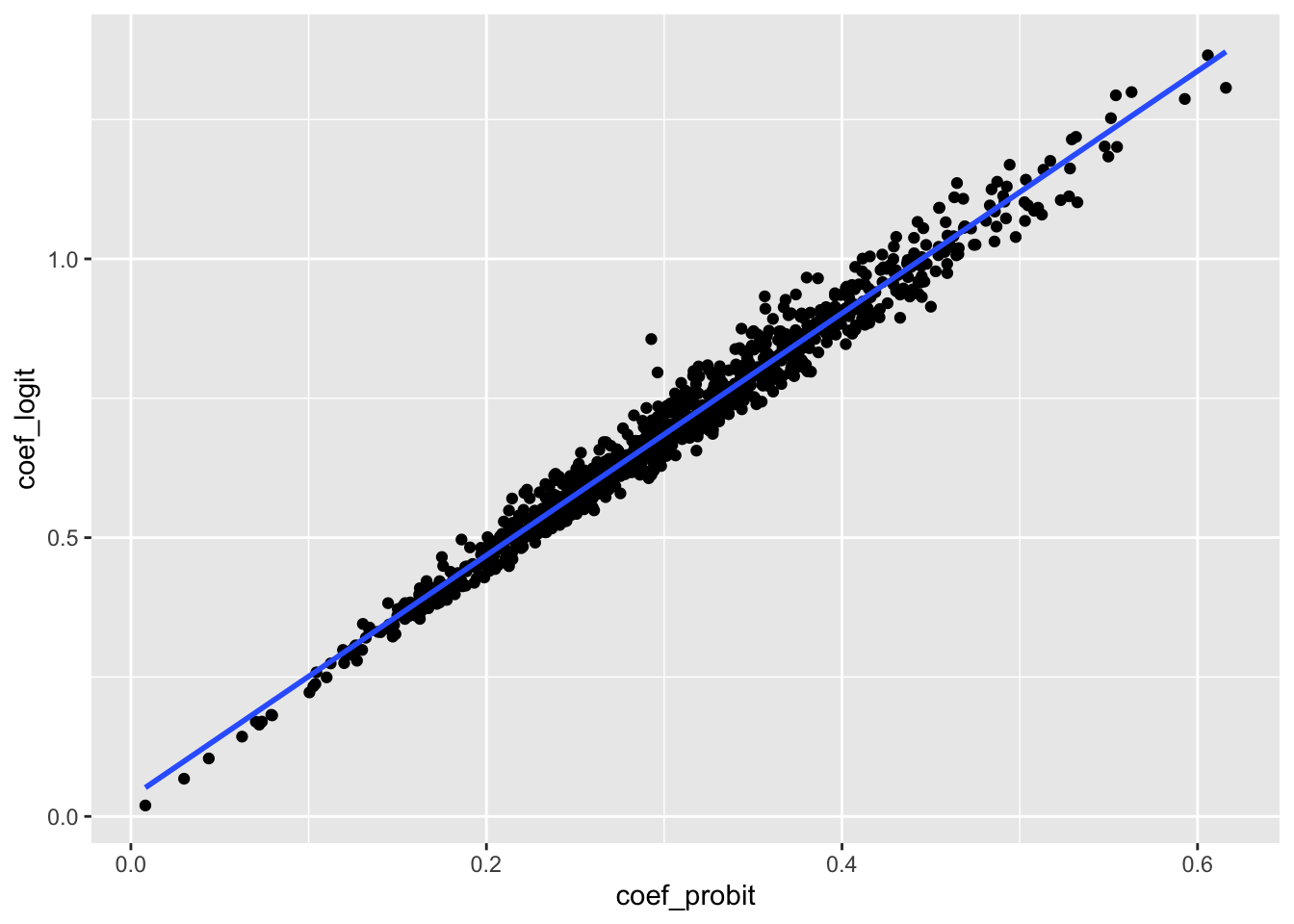
Of course, very little attention is paid to the magnitude of the coefficients from estimated probit or logit models in accounting research. While this partly reflects the focus on the statistical significance and sign of the coefficients in the NHST paradigm, it also reflects the difficulty of attaching economic meaning to the values of the coefficients. In this regard, more meaning can be placed on the marginal effect estimates.
Table 23.2 reveals that in our simulation analysis there is little difference in the estimated marginal effect sizes from the three approaches, even though only one (probit) is the correct model. The strong relationship between probit and logit fixed effects is also clear in Figure 23.2.
rel_df |>
  ggplot(aes(x = mfx_probit, y = mfx_logit)) +
  geom_point() +
  geom_smooth(formula = "y ~ x", method = "lm", se = FALSE)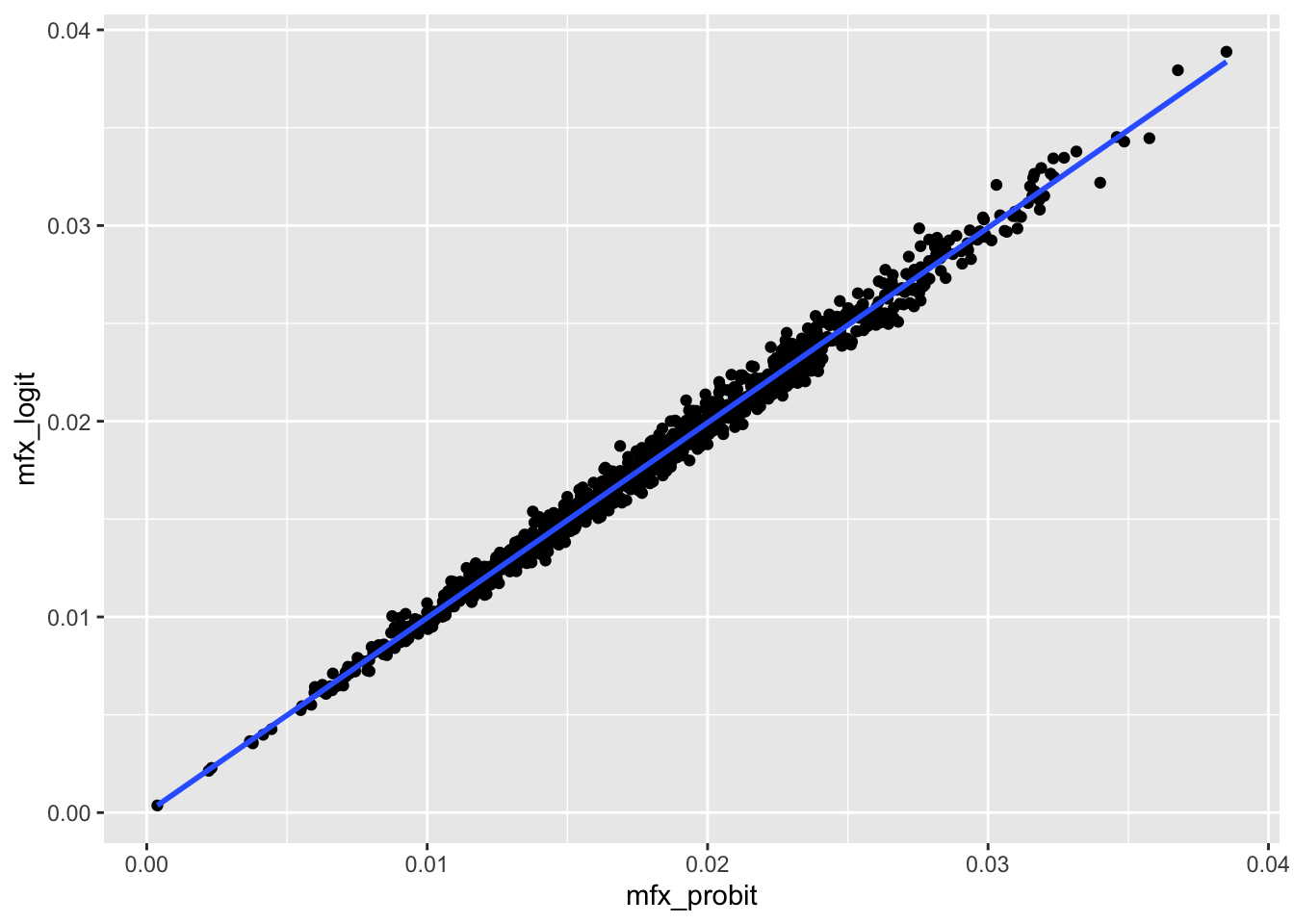
But even marginal effect sizes receive little attention in most accounting research papers, as the focus is generally on the coefficients’ signs and statistical significance. Table 23.2 provides insights on these issues too. When \(\beta_1 = 0\) (i.e., the null hypothesis is true), we see that the rejection rates are quite close to the size of the tests (either 5% or 1%) for OLS, logit, and probit and very close to each other. When \(\beta_1 = 0.3\) (i.e., the null hypothesis is false), we see that the rejection rates for OLS, logit, and probit are very similar. We have power over 90% at the 5% level and around 80% at the 1% level. As such, there is arguably little value in this setting in using probit or logit rather than OLS regression, which yields coefficients that are much easier to interpret.
| type | beta_1_true | mean_coef | mean_mfx | rej_rate_5 | rej_rate_1 |
|---|---|---|---|---|---|
| OLS | 0.0 | 0.000 | 0.000 | 0.035 | 0.008 |
| logit | 0.0 | 0.006 | 0.000 | 0.033 | 0.008 |
| probit | 0.0 | 0.002 | 0.000 | 0.035 | 0.008 |
| OLS | 0.3 | 0.018 | 0.018 | 0.938 | 0.805 |
| logit | 0.3 | 0.696 | 0.018 | 0.938 | 0.800 |
| probit | 0.3 | 0.305 | 0.018 | 0.934 | 0.801 |
Of course, the analysis above should not be assumed to apply in all settings. But it seems reasonable for deviations from straightforward OLS analysis in specific settings to be justified. Fortunately, simulation analysis like that above is relatively straightforward to conduct.
23.2.4 Count variables
Another case in which OLS may be regarded as “inadequate” is when the dependent variable is a count variable. One member of the class of GLMs that models such a dependent variable is Poisson regression. In this model, we have \(y \sim \mathrm{Pois}(\mu)\) where \(\mu = \exp(\beta_0 + \beta_1 x)\), where \(\mathrm{Pois}(\mu)\) is the Poisson distribution with parameters \(\mu\).
As above, we start by making a small function (get_pois_data()) that generates data using the assumptions underlying the Poisson model.
We then create a function to run an iteration of the simulation: get the data using get_pois_data(), extract statistics using fit_model() for both Poisson and OLS, then return a data frame with the results.
Finally, we run the simulation n_iters times for each of two values of \(\beta_1\). As above, we consider \(\beta_1 = 0\) and \(\beta_1 = 0.3\).
   user  system elapsed
  5.506   0.016   5.529
Table 23.3 reveals that in our simulation analysis there is little difference in the estimated marginal effect sizes between Poisson and OLS regression. When \(\beta_1 = 0\) (i.e., the null hypothesis is true), we see that the rejection rates are quite close to the size of the tests (either 5% or 1%) and to each other. When \(\beta_1 = 0.3\) (i.e., the null hypothesis is false), we see that the rejection rates for Poisson and OLS are very similar. Again, we have power over 90% at the 5% level and over 80% at the 1% level. As such, similar to what we saw in the analysis of probit analysis above, there is arguably little value in this setting in using Poisson regression rather than OLS regression. This seems especially true given that OLS yields coefficients that are much easier to interpret.
| type | beta_1_true | mean_coef | mean_mfx | rej_rate_5 | rej_rate_1 |
|---|---|---|---|---|---|
| OLS | 0.0 | 0.000 | 0.000 | 0.059 | 0.011 |
| Poisson | 0.0 | 0.001 | 0.000 | 0.063 | 0.010 |
| OLS | 0.3 | 0.043 | 0.043 | 0.942 | 0.849 |
| Poisson | 0.3 | 0.302 | 0.043 | 0.940 | 0.850 |
23.3 Application: Complexity and voluntary disclosure
To enrich our understanding of GLMs and to examine some additional data skills, we return to a setting similar to that considered in Guay et al. (2016). Like Guay et al. (2016), we will examine the association between complexity of financial reporting and subsequent voluntary disclosures. Our purpose here is not to conduct a close replication of Guay et al. (2016). In place of the measures of financial reporting complexity and of voluntary disclosure used in Guay et al. (2016), we use measures that are readily available. Additionally, we do not restrict ourselves to the sample period used in Guay et al. (2016).
This is the first chapter in which we need to collect a substantial amount of data from sources other than WRDS. To facilitate this, we will perform a number of data steps as quite discrete steps. This allows the re-running of code for one data set without requiring us to rerun code for other data sets.
To make this approach easier, we create save_parquet(), which takes a (possibly remote) data frame and uses the write_parquet() function from the arrow library to save it as a parquet file. The parquet format is described in R for Data Science (Wickham et al., 2023, p. 393) as “an open standards-based format widely used by big data systems.” Parquet files provide a format optimized for data analysis, with a rich type system. More details on the parquet format can be found in Chapter 22 of R for Data Science. We use write_parquet() from the arrow package to store the data in sec_index_2022q2 in a file named sec_index_2022q2.parquet.
save_parquet <- function(df, name, schema = "", path = data_dir) {
  file_path <- file.path(path, schema, str_c(name, ".parquet"))
  write_parquet(collect(df), sink = file_path)
}
23.3.1 Measures of reporting complexity
Guay et al. (2016) consider a number of measures of reporting complexity, including measures based on the “readability”, measured using the Fog index (Guay et al., 2016, p. 239), and length of a firm’s 10-K, measured as the natural logarithm of the number of words. Loughran and McDonald (2014) find “that 10-K document file size provides a simple readability proxy that outperforms the Fog Index, does not require document parsing, facilitates replication, and is correlated with alternative readability constructs.” Thus, we use 10-K document file size here.
Data on 10-K document file size can be collected from SEC EDGAR, but gathering these directly from SEC EDGAR would involve costly web scraping. Thus, we simply get these data from the website provided by Loughran and McDonald (2014).
In this book so far, we have avoided substantial data collection efforts of the kind that are often central in conducting research. From a pedagogical perspective, such data collection efforts typically involve messy details and complications that could distract more than they enlighten. However, we feel that it is useful to readers to provide some examples of more substantial data-collection tasks.
We first specify a directory in which we will store the data we will collect and create this directory if it doesn’t already exist. While the use of the DATA_DIR environment variable does not add anything in the analysis here, it may have a role if we are using local file storage across projects (see Appendix E for more on this point).5
Tip
The following line of code is only indicative. If you have already set DATA_DIR (e.g., if you have set up a data repository as discussed in Appendix E), then you may not need (or want) to run this line. If you are within an RStudio project when running the following line, then it should set DATA_DIR to a data folder inside that project, which is a reasonable choice for current purposes.
Sys.setenv(DATA_DIR = "data")data_dir <- Sys.getenv("DATA_DIR")
if (!dir.exists(data_dir)) dir.create(data_dir)Using an approach discussed in Appendix E, we will organize the data in this directory into subdirectories, which we can think of as schemas, much as data on WRDS are organized into schemas.
Specifically, we imagine that this code is being used for a hypothetical project named “glms” and we put all data specific to this project into a directory with that name. We store the full path to this directory, a subdirectory of data_dir, in project_dir.
project_dir <- file.path(data_dir, "glms")
if (!dir.exists(project_dir)) dir.create(project_dir)
It turns out that the Loughran and McDonald (2014) website provides a link to a CSV file stored in Google Drive and we can use the googledrive package to download this. This requires supplying the Google Drive ID (stored in id below) and a local file name to use (stored in lm_data below). The code below only downloads the file if it is not already present in the location stored in lm_data.6
drive_deauth()
lm_data <- file.path(project_dir, "lm_10x_summary.csv")
id <- "1puReWu4AMuV0jfWTrrf8IbzNNEU6kfpo"
if (!file.exists(lm_data)) drive_download(as_id(id), lm_data)
Having downloaded this CSV file, we can read it into R. While one way to read this file would use read_csv() from the readr package, we continue the approach of using database-backed dplyr used elsewhere in the book. However, rather than using a PostgreSQL database, we will use a local DuckDB database. DuckDB works much like PostgreSQL, but does not require a server to be set up and comes with excellent facilities for reading common file formats, such as CSV and parquet files (discussed below).
In fact, we can set up a temporary database with a single line of code:
Having created this database connection, we can use DuckDB’s native ability to read CSV files provided by its read_csv() function to create a database table as follows. We convert all variable names to lower case, convert cik to integer type and filing_date and cpr to date types, and handle the -99 value used to represent missing values in cpr. (According to the source website, cpr refers to the “conformed period of report” of the filing, which is the last date of the reporting period.)
Note that we force the table to be materialized as a remote temporary table by appending the command compute(). This takes less than a second, but means that the conversion from CSV and processing of dates and missing values and the like happens only once rather than each time we call on lm_10x_summary in later analyses. Judicious use of compute() can also enhance query performance even when a table is not used multiple times by making it easier for the query optimizer in our database to understand the query. Unfortunately, WRDS does not grant its users sufficient privileges to create temporary tables and thus we have not been able to use compute() in previous chapters.7
lm_10x_summary <-
  tbl(db, str_c("read_csv('", lm_data, "')")) |>
  rename_with(tolower) |>
  mutate(cik = as.integer(cik),
         filing_date = as.character(filing_date),
         cpr = if_else(cpr == -99, NA, as.character(cpr))) |>
  mutate(filing_date = as.Date(strptime(filing_date, '%Y%m%d')),
         cpr = as.Date(strptime(cpr, '%Y%m%d'))) |>
  compute()
This remote table lm_10x_summary is just like the remote tables we first saw in Section 6.1.
lm_10x_summary# Source: table<dbplyr_if0zhyOp7u> [?? x 26]
# Database: DuckDB 1.5.2 [root@Darwin 27.0.0:R 4.6.0/:memory:]
cik filing_date acc_num cpr form_type coname sic ffind n_words
<int> <date> <chr> <date> <chr> <chr> <dbl> <dbl> <dbl>
1 60512 1993-08-13 000006… 1993-06-30 10-Q LOUIS… 1311 30 4068
2 66740 1993-08-13 000006… 1993-06-30 10-Q MINNE… 2670 38 4389
3 60512 1993-10-07 000006… 1992-12-31 10-K-A LOUIS… 1311 30 8719
4 60512 1993-11-10 000006… 1993-09-30 10-Q LOUIS… 1311 30 4938
5 11860 1993-11-12 000001… 1993-09-30 10-Q BETHL… 3312 19 3823
6 20762 1993-11-12 000095… 1993-09-30 10-Q CLARK… 2911 30 4136
# ℹ more rows
# ℹ 17 more variables: n_unique_words <dbl>, n_negative <dbl>,
# n_positive <dbl>, n_uncertainty <dbl>, n_litigious <dbl>,
# n_strongmodal <dbl>, n_weakmodal <dbl>, n_constraining <dbl>,
# n_complexity <dbl>, n_negation <dbl>, grossfilesize <dbl>,
# netfilesize <dbl>, nontextdoctypechars <dbl>, htmlchars <dbl>,
# xbrlchars <dbl>, xmlchars <dbl>, n_exhibits <dbl>From a quick inspection, we can see that the data begin in 1993, but only appear to be comprehensive from some time in 1995 or 1996.
# A tibble: 31 × 2
   year     n
  <dbl> <dbl>
1  1993    13
2  1994  9752
3  1995 21880
4  1996 44531
5  1997 55484
6  1998 55735
# ℹ 25 more rows
Finally, we save the data to a parquet file in our glms project directory and disconnect from the in-memory DuckDB database.
lm_10x_summary |>
  save_parquet(name = "lm_10x_summary", schema = "glms")

dbDisconnect(db)
23.3.2 Data on EDGAR filings
As discussed above, Guay et al. (2016) consider a number of measures of voluntary disclosure. While measures based on management forecasts require data from IBES and measures of firm-initiated press releases require data from RavenPack, the measure based on the number of 8-Ks filed in a period can be collected from SEC EDGAR fairly easily and we focus on that measure for this reason.
Here we collect filings data from SEC EDGAR. Specifically, we collect index files for each quarter. These index files include details on each filing in the applicable quarter.
For example, if you visit https://www.sec.gov/Archives/edgar/full-index/2022/QTR2/, you can see a number of files available to download. As these files are mostly different ways of presenting the same information in a variety of formats, we will focus on the company.gz files.
The first practical challenge we face is that if we try to use download.file() to get company.gz, we will get a “403 Forbidden” error message because the SEC does not allow anonymous downloads. To avoid this, we set the HTTPUserAgent option using our email address (obviously, use your actual email address here).
options(HTTPUserAgent = "your_name@some_email.com")The file company.gz is a compressed fixed-width format text file of the kind examined in Chapter 9.
url <- str_c("https://www.sec.gov/Archives/edgar/full-index/",
             "2022/QTR2/company.gz")
t <- tempfile(fileext = ".gz")
download.file(url, t)

sec_index_2022q2 <-
  read_fwf(t,
           fwf_cols(company_name = c(1, 62),
                    form_type = c(63, 77),
                    cik = c(78, 89),
                    date_filed = c(90, 101),
                    file_name = c(102, NA)),
           col_types = "cciDc",
           skip = 10,
           locale = locale(encoding = "macintosh"))
sec_index_2022q2 |> select(company_name, cik)# A tibble: 291,648 × 2
company_name cik
<chr> <int>
1 006 - Series of IPOSharks Venture Master Fund, LLC 1894348
2 008 - Series of IPOSharks Venture Master Fund, LLC 1907507
3 01 Advisors 03, L.P. 1921173
4 01Fintech LP 1928541
5 07 Carbon Capture, LP 1921663
6 09 Carbon Capture, LP 1936048
# ℹ 291,642 more rowssec_index_2022q2 |> select(form_type, date_filed, file_name)# A tibble: 291,648 × 3
form_type date_filed file_name
<chr> <date> <chr>
1 D 2022-04-08 edgar/data/1894348/0001892986-22-000003.txt
2 D 2022-06-07 edgar/data/1907507/0001897878-22-000003.txt
3 D 2022-05-20 edgar/data/1921173/0001921173-22-000001.txt
4 D 2022-05-13 edgar/data/1928541/0001928541-22-000001.txt
5 D 2022-04-05 edgar/data/1921663/0001921663-22-000001.txt
6 D 2022-06-30 edgar/data/1936048/0001936048-22-000001.txt
# ℹ 291,642 more rowsAs the file we downloaded above is over 4 MB in size and we will need to download dozens of such files, we likely want to store these data in some permanent fashion. While one approach would be to use a PostgreSQL database to which we have write access, we do not assume here that you have such a database.8
Another approach would be to simply download all the company.gz files and process them each time we use them. The problem with this approach is that this processing is time-consuming and thus best done once.
Here we use the parquet file format to store the data. As it is easy to imagine using these on projects other than our hypothetical "glms" project, we will store the SEC EDGAR filings data discussed in edgar, a subdirectory of DATA_DIR defined above.
edgar_dir <- file.path(data_dir, "edgar")
if (!dir.exists(edgar_dir)) dir.create(edgar_dir)
sec_index_2022q2 |>
  save_parquet("sec_index_2022q2", schema = "edgar")
This parquet file can be read into R in many ways. For example, we could use the open_dataset() function from the arrow library. However, we will use a DuckDB database connection db—created using a single line of code below—and the DuckDB-specific load_parquet() function provided by the farr package to create a database table.9
db <- dbConnect(duckdb::duckdb())

sec_index <- load_parquet(db, "sec_index_2022q2", schema = "edgar")
If we were using just a single index file, the benefits of using DuckDB rather than the open_dataset() function might be less clear. However, we will soon see how easy it is to work with parquet files using DuckDB and also look to combine these index files with the data in the lm_10x_summary data frame we created above and data from Compustat and CRSP.
Our next step is to embed the code we used above to download and process company.gz for a single quarter in a function that can download an SEC index file and save it as a parquet file. Armed with this function, we can then process multiple index files in one step. Naturally, the function we create below (get_sec_index()) addresses possibilities ignored above, such as download failures.
get_sec_index <- function(year, quarter, overwrite = FALSE) {

  pq_path <- str_c(edgar_dir, "/sec_index_",
                    year, "q", quarter, ".parquet")
  if (file.exists(pq_path) & !overwrite) return(TRUE)

  # Download the zipped index file from the SEC website
  url <- str_c("https://www.sec.gov/Archives/edgar/full-index/",
               year,"/QTR", quarter, "/company.gz")

  t <- tempfile(fileext = ".gz")
  result <- try(download.file(url, t))

  # If we didn't encounter an error downloading the file, parse it
  # and save as a parquet file
  if (!inherits(result, "try-error")) {
    temp <-
      read_fwf(t, fwf_cols(company_name = c(1, 62),
                           form_type = c(63, 77),
                           cik = c(78, 89),
                           date_filed = c(90, 101),
                           file_name = c(102, NA)),
               col_types = "ccicc", skip = 10,
               locale = locale(encoding = "macintosh")) |>
      mutate(date_filed = as.Date(date_filed))

    write_parquet(temp, sink = pq_path)
    return(TRUE)
  } else {
    return(FALSE)
  }
}
We next create a data frame containing the years and quarters for which we want to collect SEC index files. SEC EDGAR extends back to 1993 and index files for the current quarter will appear after the first day of the quarter. We can use the crossing() function from the tidyr package to create the Cartesian product of the quarters and years.
Finally, we can download the SEC index files using the following few lines of code.
Tip
The following code takes several minutes to run. This code took us around 4 minutes to run, but the time required will depend on things such as the speed of your internet connection.
After running the code above, we have 132 index files saved as parquet files in edgar_dir occupying 5 MB of drive space. This represents much more than 5 MB of data because parquet files are highly compressed.
Reading these data into our database is simple and quick. We can use a wildcard to combine several parquet files ("sec_index*.parquet" here) into a single table.
sec_index <- load_parquet(db, "sec_index*", "edgar")We can check that we have data for 132 quarters. As we saw above with the data on 10-Ks, there are few observations in 1993 and a significant increase from 1994 to 1995.
# A tibble: 1 × 3
   year quarter      n
  <dbl>   <dbl>  <dbl>
1  2022       2 291648
Each filing on SEC EDGAR has a form_type. As can be seen in Table 23.4, the most common form type is Form 4, which is filed whenever there is a material change in the holdings of company insiders. The second most common form type is Form 8-K, which the SEC describes as “the ‘current report’ companies must file with the SEC to announce major events that shareholders should know about.”
| form_type | n |
|---|---|
| 4 | 105,830 |
| 424B2 | 24,753 |
| 8-K | 19,320 |
| NPORT-P | 12,676 |
| D | 11,029 |
| 3 | 7,736 |
| 6-K | 7,430 |
| 13F-HR | 6,841 |
| 10-Q | 6,610 |
| FWP | 5,827 |
As mentioned above, we will construct a measure of disclosure based on the number of 8-K filings. While 8-K filings represent the second-most common form of filing, they are still a small share of all filings. Figure 23.3 shows some clear trends in the number of filings over time. Form 8-K filings appear to have peaked in number in 2005 and to have been in slow decline in number since then.
sec_index |>
  mutate(year = year(date_filed),
         form_type = if_else(form_type %in% c("4", "8-K"),
                             form_type, "Other")) |>
  filter(year < max(year, na.rm = TRUE)) |>
  count(year, form_type) |>
  mutate(last_year =  year == max(year, na.rm = TRUE),
         label = if_else(last_year, form_type, NA)) |>
  ggplot(aes(x = year, y = n / 1000,
             colour = form_type, linetype = form_type)) +
  geom_line() +
  geom_label(aes(label = label), na.rm = TRUE,
             position = position_nudge(y = -0.4)) +
  scale_y_continuous(name = "Number of filings (thousands)") +
  scale_x_continuous(breaks = seq(1993, current_year, 2)) +
  theme(axis.text.x = element_text(angle = 90),
        legend.position = "none")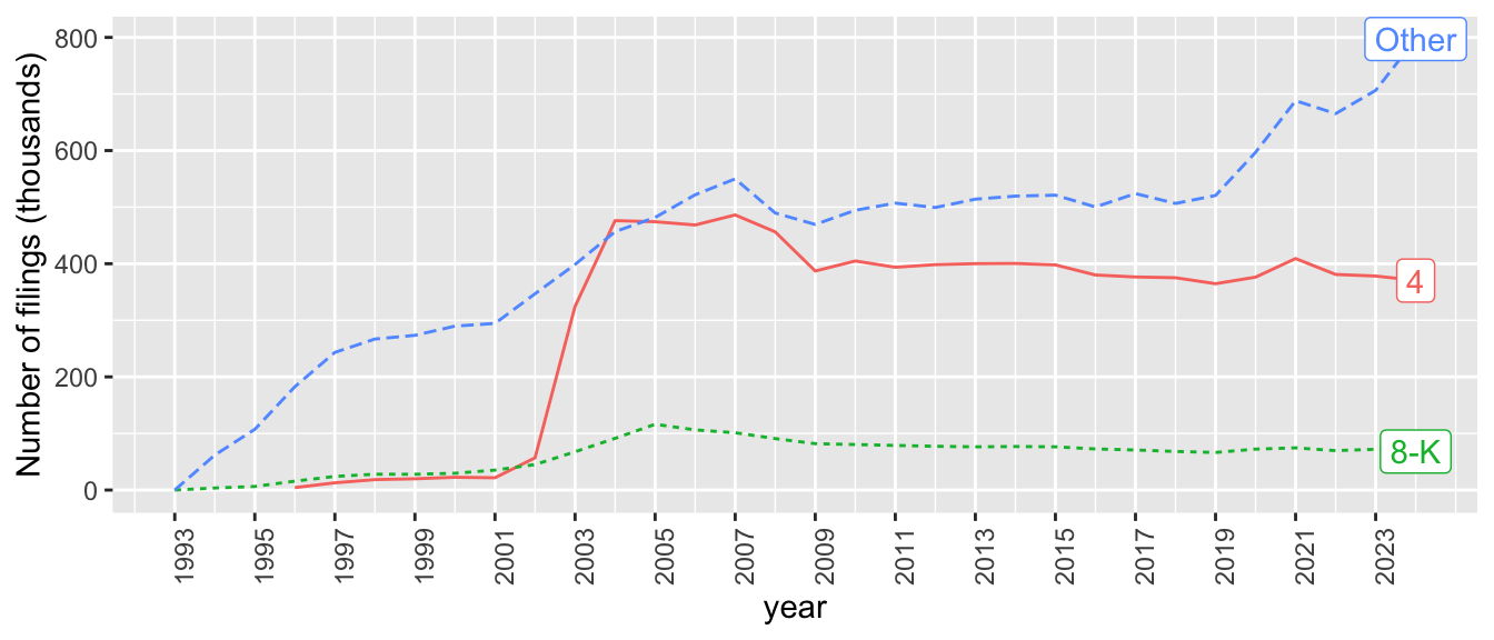
One thing to note about SEC form types is that there are often variants on basic form types. For example, 8-K/A indicates an amended 8-K filing. We can identify the variants using regular expressions. In the case of 8-K filings, it appears from Table 23.5 that the vast majority are on the base 8-K form type.
| form_type | n | percent |
|---|---|---|
| 8-K | 19,320 | 97.689 |
| 8-K/A | 444 | 2.245 |
| 8-K12B | 9 | 0.046 |
| 8-K12B/A | 2 | 0.010 |
| 8-K12G3 | 2 | 0.010 |
dbDisconnect(db)23.3.3 Measure of financial statement complexity
Our analysis below will take as the basic unit of observation the filing of a 10-K by a firm and examine the level of voluntary disclosure around that 10-K filing as a function of its complexity.
While lm_10x_summary contains many metrics related to filings, we retain only acc_num, cik, the two date columns (filing_date and cpr), and the grossfilesize column in our table filing_10k_merged.
As we will following Guay et al. (2016) in including a number of controls calculated using data from Compustat (and CRSP), we need to link each 10-K filing to a GVKEY. To do so, we will use the gvkey_ciks table included in the farr package.
The gvkey_ciks table includes links between gvkey-idd combinations and cik values along with the range of dates (first_date to last_date) for which the links are valid. We join the lm_10x_summary table containing data on 10-K filings with gvkey_ciks using the common field cik when filing_date is between first_date and last_date. As the lm_10x_summary table containing data on 10-K filings is a remote table inside our DuckDB database and the gvkey_ciks is a local data frame, we need to copy the latter to the database using copy = TRUE.
db <- dbConnect(duckdb::duckdb())

lm_10x_summary <- load_parquet(db, "lm_10x_summary", schema = "glms")

filing_10k_merged <-
  lm_10x_summary |>
  filter(form_type == "10-K") |>
  inner_join(gvkey_ciks,
             join_by(cik, between(filing_date, first_date, last_date)),
             copy = TRUE) |>
  select(gvkey, iid, acc_num, cik, filing_date, cpr, grossfilesize) |>
  mutate(eomonth = floor_date(cpr, "month") + months(1) - days(1)) |>
  save_parquet(name = "filing_10k_merged", schema = "glms")

dbDisconnect(db)
23.3.4 Measure of voluntary disclosure
We can now move on to constructing our measure of voluntary disclosure. We start by creating filing_8k, which only includes 8-K filings. We rename date_filed to date_8k to avoid confusion that might arise when we combine with data on 10-Ks that have their own filing dates.
db <- dbConnect(duckdb::duckdb())
sec_index <- load_parquet(db, "sec_index*", "edgar")We then combine filing_10k_merged with filing_8k using CIK and keep all 8-K filings between one year before and one year after the 10-K filing date. We rename filing_date as fdate in part to shorter lines of code. Having constructed this merged table, we then count the number of 8-K filings within various windows (e.g., between(datediff, 0, 30) represents 8-K filings in the 30-day window starting on the date of the 10-K filing.10
It is noteworthy that this code runs in less than a second on our computer, illustrating the performance benefits of DuckDB. If the source tables (filing_10k_merged and filing_8k) are instead converted to local data frames using collect(), this query takes nearly a minute.
Because the arguments to between() are “out of order” in that date_8k comes from filing_8k, the second table referred to in inner_join(), we indicate this by qualifying it with y$ and that fdate_m1 and fdate_p1 come from filing_10k_merged by qualifying these with x$.
filing_10k_merged <- load_parquet(db, "filing_10k_merged", schema = "glms")

vdis_df <-
  filing_10k_merged |>
  rename(fdate = filing_date) |>
  mutate(fdate_p1 = fdate + years(1L),
         fdate_m1 = fdate - years(1L)) |>
  inner_join(filing_8k,
             join_by(cik,
                     between(y$date_8k, x$fdate_m1, x$fdate_p1))) |>
  mutate(datediff = as.double(date_8k - fdate)) |>
  group_by(acc_num, gvkey, iid, cik) |>
  summarize(vdis_p1y = sum(as.integer(datediff > 0)),
            vdis_p30 = sum(as.integer(between(datediff, 0, 30))),
            vdis_p60 = sum(as.integer(between(datediff, 0, 60))),
            vdis_p90 = sum(as.integer(between(datediff, 0, 90))),
            vdis_m1y = sum(as.integer(datediff < 0)),
            vdis_m30 = sum(as.integer(between(datediff, -30, -1))),
            vdis_m60 = sum(as.integer(between(datediff, -60, -1))),
            vdis_m90 = sum(as.integer(between(datediff, -90, -1))),
            .groups = "drop") |>
  group_by(acc_num, gvkey, iid) |>
  filter(vdis_p1y == max(vdis_p1y, na.rm = TRUE)) |>
  ungroup() |>
  save_parquet(name = "vdis_df", schema = "glms")

dbDisconnect(db)
23.3.5 Controls
In addition to our measure of voluntary disclosure (in vdis_df) and our measure of financial statement complexity (in filing_10k_merged), we need data on various controls for our empirical analysis. These controls are based on Guay et al. (2016) and the required data come from Compustat and CRSP.
Thus, as in previous chapters, we will collect these data from the WRDS PostgreSQL database. However, we take a different approach to data collection in this chapter from the approaches we have used in earlier chapters.
For example, in Chapter 12, we had a relatively small amount of data on earnings announcement dates in a local data frame. When we needed to combine those event dates with data from CRSP, we simply copied the data to the WRDS server using the copy_inline() function, then summarized the data into a smaller data set using the WRDS PostgreSQL server, then used collect() to retrieve the data for further empirical analysis. This approach will not work well when our local data frame is too large to work well with copy_inline().11
The approach we use in this chapter does not require sending large amounts of data to the CRSP PostgreSQL server. Additionally, we use persistent storage (specifically parquet files) to make it easier to break our analysis into discrete steps that do not require the rerunning of costly earlier data steps each time we start R.
The data sets we need to collect from WRDS are:
- Fundamental data from
comp.funda. - Data on event dates for GVKEYs derived from
crsp.dsiandcrsp.ccmxpf_lnkhist. - Data on “trading dates” derived from
crsp.dsi. (See Chapter 13 for more details.) - Data on liquidity measures derived from
crsp.dsf.
For each of these four data sets, we will perform the following steps.
- Connect to the database server.
- Create a remote data frame for the underlying table.
- Process the data as needed using
dplyrverbs. - Save the resulting data as a parquet file.
- Close the connection to the database server.
23.3.5.1 Fundamental data from comp.funda
We start with fundamental data and indicators for relevance of SFAS 133 and SFAS 157, as discussed in Guay et al. (2016) and papers cited therein, and store these as compustat.
db <- dbConnect(RPostgres::Postgres())

funda <- tbl(db, Id(schema = "comp", table = "funda"))

compustat <-
  funda |>
  filter(indfmt == 'INDL', datafmt == 'STD',
         popsrc == 'D', consol == 'C') |>
  mutate(mkt_cap = prcc_f * csho,
         size = if_else(mkt_cap > 0, log(mkt_cap), NA),
         roa = if_else(at > 0, ib / at, NA),
         mtb = if_else(ceq > 0, mkt_cap / ceq, NA),
         special_items = if_else(at > 0, coalesce(spi, 0) / at, NA),
         fas133 = !is.na(aocidergl) & aocidergl != 0,
         fas157 = !is.na(tfva) & tfva != 0) |>
  select(gvkey, iid, datadate, mkt_cap, size, roa, mtb,
         special_items, fas133, fas157) |>
  filter(mkt_cap > 0) |>
  mutate(eomonth = floor_date(datadate, "month") + months(1) - days(1)) |>
  save_parquet(name = "compustat", schema = "glms")

dbDisconnect(db)
db <- dbConnect(duckdb::duckdb())
funda <- load_parquet(db, schema = "comp", table = "funda")
compustat <-
funda |>
filter(indfmt == 'INDL', datafmt == 'STD',
popsrc == 'D', consol == 'C') |>
mutate(mkt_cap = prcc_f * csho,
size = if_else(mkt_cap > 0, log(mkt_cap), NA),
roa = if_else(at > 0, ib / at, NA),
mtb = if_else(ceq > 0, mkt_cap / ceq, NA),
special_items = if_else(at > 0, coalesce(spi, 0) / at, NA),
fas133 = !is.na(aocidergl) & aocidergl != 0,
fas157 = !is.na(tfva) & tfva != 0) |>
select(gvkey, iid, datadate, mkt_cap, size, roa, mtb,
special_items, fas133, fas157) |>
filter(mkt_cap > 0) |>
mutate(eomonth = floor_date(datadate, "month") + months(1) - days(1)) |>
save_parquet(name = "compustat", schema = "glms")
dbDisconnect(db)23.3.5.2 Data on event dates for GVKEYs
Next, we create the data frame event_dates that will contain permno, start_date and end_date for each of our events (10-K filing dates). The logic here is similar to that we saw in constructing event dates for Apple media events in Chapter 13 and we use the now-familiar ccm_link table that we first saw in Section 7.3.
pg <- dbConnect(RPostgres::Postgres())
db <- dbConnect(duckdb::duckdb())

ccmxpf_lnkhist <- tbl(pg, Id(schema = "crsp", table = "ccmxpf_lnkhist"))
filing_10k_merged <- load_parquet(db, table = "filing_10k_merged",
                               schema = "glms")
ccm_link <-
  ccmxpf_lnkhist |>
  filter(linktype %in% c("LC", "LU", "LS"),
         linkprim %in% c("C", "P")) |>
  mutate(linkenddt = coalesce(linkenddt, max(linkenddt, na.rm = TRUE))) |>
  rename(permno = lpermno,
         iid = liid) |>
  copy_to(db, df = _, name = "ccm_link", overwrite = TRUE)

filing_permnos <-
  filing_10k_merged |>
  inner_join(ccm_link,
             join_by(gvkey, iid,
                     between(filing_date, linkdt, linkenddt))) |>
  select(gvkey, iid, filing_date, permno)

event_dates <-
  filing_permnos |>
  distinct(permno, filing_date) |>
  collect() |>
  get_event_dates(pg, permno = "permno",
                  event_date = "filing_date",
                  win_start = -20, win_end = 20) |>
  copy_to(db, df = _, name = "event_dates", overwrite = TRUE) |>
  inner_join(filing_permnos, by = join_by(permno, filing_date)) |>
  save_parquet(name = "event_dates", schema = "glms")

dbDisconnect(pg)
dbDisconnect(db)
db <- dbConnect(duckdb::duckdb())
ccmxpf_lnkhist <- load_parquet(db, schema = "crsp", table = "ccmxpf_lnkhist")
filing_10k_merged <- load_parquet(db, table = "filing_10k_merged",
schema = "glms")
ccm_link <-
ccmxpf_lnkhist |>
filter(linktype %in% c("LC", "LU", "LS"),
linkprim %in% c("C", "P")) |>
mutate(linkenddt = coalesce(linkenddt, max(linkenddt, na.rm = TRUE))) |>
rename(permno = lpermno,
iid = liid) |>
copy_to(db, df = _, name = "ccm_link", overwrite = TRUE)
filing_permnos <-
filing_10k_merged |>
inner_join(ccm_link,
join_by(gvkey, iid,
between(filing_date, linkdt, linkenddt))) |>
select(gvkey, iid, filing_date, permno)
event_dates <-
filing_permnos |>
distinct(permno, filing_date) |>
collect() |>
get_event_dates(pg, permno = "permno",
event_date = "filing_date",
win_start = -20, win_end = 20) |>
copy_to(db, df = _, name = "event_dates", overwrite = TRUE) |>
inner_join(filing_permnos, by = join_by(permno, filing_date)) |>
save_parquet(name = "event_dates", schema = "glms")
dbDisconnect(db)23.3.5.3 Data on “trading dates”
We first saw the trading_dates table in Chapter 12 and we use the get_trading_dates() function from the farr package to create that using data from the WRDS PostgreSQL database and then save it as a parquet file.
db <- dbConnect(RPostgres::Postgres())

trading_dates <-
  get_trading_dates(db) |>
  save_parquet(name = "trading_dates", schema = "glms")

dbDisconnect(db)
db <- dbConnect(duckdb::duckdb())
trading_dates <-
get_trading_dates(db) |>
save_parquet(name = "trading_dates", schema = "glms")
dbDisconnect(db)23.3.5.4 Data on liquidity measures
A core idea of Guay et al. (2016) is that firms use voluntary disclosure to mitigate the deleterious effects of financial statement complexity. One of the costs of greater financial statement complexity is greater illiquidity (i.e., less liquidity) in the market for a firm’s equity. Guay et al. (2016) examine two primary measures of liquidity: the “Amihud (2002) measure” and the bid-ask spread. The following code calculates these measures using the formulas provided by Guay et al. (2016, p. 240).
Tip
The following code takes several minutes to run because a large about of data needs to be downloaded from crsp.dsf. This code took us nearly 4 minutes to run, but the time required will depend on things such as the speed of your internet connection.
pg <- dbConnect(RPostgres::Postgres())
db <- dbConnect(duckdb::duckdb())

dsf <- tbl(pg, Id(schema = "crsp", table = "dsf"))
filing_10k_merged <- load_parquet(db, "filing_10k_merged", schema = "glms")

first_year <-
  filing_10k_merged |>
  summarize(min(year(filing_date)) - 1L) |>
  pull()

last_year <-
  filing_10k_merged |>
  summarize(max(year(filing_date)) + 1L) |>
  pull()

liquidity <-
  dsf |>
  filter(between(year(date), first_year, last_year)) |>
  mutate(prc = abs(prc),
         spread = if_else(prc > 0, (ask - bid) / prc, NA),
         illiq = if_else(vol * prc > 0, abs(ret) / (vol * prc), NA)) |>
  mutate(spread = spread * 100,
         illiq = illiq * 1e6) |>
  filter(!is.na(spread), !is.na(illiq)) |>
  select(permno, date, spread, illiq) |>
  save_parquet(name = "liquidity", schema = "glms")

dbDisconnect(pg)
dbDisconnect(db)
db <- dbConnect(duckdb::duckdb())
dsf <- load_parquet(db, schema = "crsp", table = "dsf")
filing_10k_merged <- load_parquet(db, "filing_10k_merged",
schema = "glms")
first_year <-
filing_10k_merged |>
summarize(min(year(filing_date)) - 1L) |>
pull()
last_year <-
filing_10k_merged |>
summarize(max(year(filing_date)) + 1L) |>
pull()
liquidity <-
dsf |>
filter(between(year(date), first_year, last_year)) |>
mutate(prc = abs(prc),
spread = if_else(prc > 0, (ask - bid) / prc, NA),
illiq = if_else(vol * prc > 0, abs(ret) / (vol * prc), NA)) |>
mutate(spread = spread * 100,
illiq = illiq * 1e6) |>
filter(!is.na(spread), !is.na(illiq)) |>
select(permno, date, spread, illiq) |>
save_parquet(name = "liquidity", schema = "glms")
dbDisconnect(db)23.3.6 Empirical analysis
Now that we have collected all the data we need, we can run the final analysis. We can load the parquet data created in the previous section using the load_parquet() function made available by the farr package.
db <- dbConnect(duckdb::duckdb())

vdis_df <- load_parquet(db, table = "vdis_df", schema = "glms")
filing_10k_merged <- load_parquet(db, table = "filing_10k_merged",
                                  schema = "glms")
liquidity <- load_parquet(db, table = "liquidity", schema = "glms")
trading_dates <- load_parquet(db, table = "trading_dates", schema = "glms")
event_dates <- load_parquet(db, table = "event_dates", schema = "glms")
compustat <- load_parquet(db, table = "compustat", schema = "glms")
We combine event dates with liquidity data.
Because the arguments to between() are again “out of order”, in joining event_dates and liquidity, we indicate the source tables with x$ and y$. We then use trading_dates to match each filing_date and each date with a trading date (td) value.
liquidity_merged <-
  event_dates |>
  inner_join(liquidity,
             join_by(permno,
                     between(y$date, x$start_date, x$end_date))) |>
  inner_join(trading_dates, join_by(filing_date == date)) |>
  rename(filing_td = td) |>
  inner_join(trading_dates, join_by(date)) |>
  mutate(rel_td = td - filing_td) |>
  select(gvkey, iid, permno, filing_date, rel_td, spread, illiq) |>
  compute()
Some analyses in Guay et al. (2016) reduce complexity measures to either quintiles or deciles and we use quintiles for the complexity measure here. To allow for secular changes in complexity over time, we form quintiles by the year of filing_date.
Like Guay et al. (2016), we impose a sample requirement of complete data (i.e., 20 trading days) prior to the filing of the 10-K.
To better understand the underlying relations in the data, we examine the behaviour of measures of illiquidity around event dates by complexity quintile. We form deciles by year for the two measures of illiquidity. To facilitate plotting, we use pivot_longer() and convert complex_q5 from a numeric to a character variable.12
plot_data <-
  complexity |>
  inner_join(liquidity_merged,
             by = join_by(gvkey, iid, filing_date)) |>
  semi_join(complete_cases,
            by = join_by(gvkey, iid, filing_date)) |>
  group_by(year) |>
  mutate(spread = ntile(spread, 10),
         illiq = ntile(illiq, 10)) |>
  group_by(rel_td, complex_q5) |>
  summarize(spread = mean(spread, na.rm = TRUE),
            illiq = mean(illiq, na.rm = TRUE),
            num_obs = n(),
            .groups = "drop") |>
  pivot_longer(spread:illiq, names_to = "measure") |>
  mutate(complex_q5 = as.character(complex_q5)) |>
  compute()
Once we have structured the data appropriately, creation of the plot seen in Figure 23.4 requires just a few lines of code.
plot_data |>
  mutate(last_day =  rel_td == max(rel_td),
         label = if_else(last_day, as.character(complex_q5), NA)) |>
  ggplot(aes(x = rel_td,
             y = value,
             color = complex_q5,
             group = complex_q5)) +
  geom_line() +
  geom_label(aes(label = label), na.rm = TRUE) +
  facet_wrap( ~ measure) +
  theme(legend.position = "none")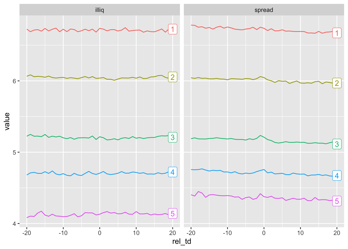
To conduct regression analysis analogous to that in Table 3 of Guay et al. (2016), we combine our data on voluntary disclosure (vdis_df) with our data on financial statement complexity (filing_10k_merged) and controls (compustat).
reg_data_glms <-
  vdis_df |>
  inner_join(filing_10k_merged,
             by = join_by(acc_num, gvkey, iid, cik)) |>
  inner_join(compustat, by = join_by(gvkey, iid, eomonth)) |>
  mutate(ln_grossfilesize = log(grossfilesize)) |>
  collect()
We run three regressions. The first two are, following Guay et al. (2016), OLS with and without firm fixed effects. The third regression is Poisson regression.
controls <- c("mkt_cap", "size", "roa", "mtb", "special_items")

model <- str_c("vdis_p1y ~ ",
                str_c(c("ln_grossfilesize", controls),
                      collapse = " + "))

fms <- list(
  "OLS" = feols(as.formula(model), data = reg_data_glms),
  "Firm FE" = feols(as.formula(str_c(model, " | gvkey + iid")),
              data = reg_data_glms),
  "Pois" = glm(as.formula(model), family = "poisson", data = reg_data_glms))
We make a small function that returns “robust” standard errors if the model is estimated using glm() (as in Poisson regression). Based on papers we examine in Chapter 24, use of robust standard errors seems to be a standard practice with Poisson regression.
Regression results are shown in Table 23.6.
modelsummary(map(fms, get_coefs),
             statistic = "statistic",
             gof_map = "nobs",
stars = c('*' = .1, '**' = 0.05, '***' = .01))| OLS | Firm FE | Pois | |
|---|---|---|---|
| * p < 0.1, ** p < 0.05, *** p < 0.01 | |||
| (Intercept) | 1.982*** | 0.631 | |
| (2.928) | (1.545) | ||
| ln_grossfilesize | -0.060 | -0.693*** | -0.032 |
| (-1.388) | (-5.326) | (-1.241) | |
| mkt_cap | -0.000* | 0.000** | -0.000** |
| (-1.949) | (2.484) | (-2.017) | |
| size | 0.107*** | 2.142*** | 0.064*** |
| (8.261) | (32.186) | (8.607) | |
| roa | -0.151*** | -0.226* | -0.103*** |
| (-2.970) | (-1.733) | (-3.150) | |
| mtb | -0.000 | -0.000*** | -0.000 |
| (-0.232) | (-3.511) | (-0.347) | |
| special_items | 0.194** | 0.307* | 0.137** |
| (2.096) | (1.719) | (2.145) | |
| Num.Obs. | 8324 | 7708 | 8324 |
Once we are done with our in-memory DuckDB database, we can disconnect from it.
dbDisconnect(db)23.3.7 Exercises
Instead of
tbl(db, sql(lm_10x_summary_sql)), we could use have usedread_csv(lm_data, show_col_types = FALSE). What benefits do you see from using the former option? (Hint: Try both versions of the code and perhaps usesystem.time()to evaluate processing times.)What primary key could we use for
lm_10x_summary? Check that this is a valid primary key.What primary key could we use for
filing_10k_merged? Check that this is a valid primary key.From Figure 23.4, do you observe a change in measures of liquidity around 10-K filing dates? Why (or why not) would we expect to see a change around these events?
From Figure 23.4, do you observe a relation between the complexity of financial statements and illiquidity? Is the sign of any relationship consistent with what we would expect from reading Guay et al. (2016)? Does the nature of the relationship affect how you interpret the results of Guay et al. (2016)?
Calculate the marginal effects associated with the regression coefficients shown in Table 23.6. Do you observe significant differences across specifications? (Hint: The
mfx()function should be able to do most of the work here.)
23.4 Further reading
Chapter 13 of Wooldridge (2010) provides a more thorough discussion of MLE. Chapter 15 of Wooldridge (2010) covers probit and logit, including MLE and marginal effects. Chapter 19 of Wooldridge (2010) covers count models, including Poisson regression. We demonstrated that OLS works well for practical purposes with simulated data, Angrist and Pischke (2008) also highlight the benefits of OLS and show that it delivers very similar inferences in a particular setting.
For more on the GLMs, including details about estimation of coefficients and standard errors, see Dunn and Smyth (2018). Aronow and Miller (2019) provide a modern take on MLE estimation.
More details on the parquet format can be found in Chapter 22 of R4DS. Chapter 19 of R4DS discusses Cartesian products.
23.5 Appendix: Maintaining a repository of SEC index files
In Section 23.3.4 we described how one can download the SEC index files and create a repository of parquet files that can be used to identify and locate filings on SEC EDGAR. Because these files are continually being updated, we might want to update our files too. However, ideally we would avoid downloading files that we already have.
If you visit any of pages from which we obtained the filings, such as the page for the second quarter of 2022 that we looked at earlier in the chapter, you can see that the “last modified” timestamp for each file.13 We can collect this information and store it and then later on only download files with a more recent “last modified” timestamp.
The get_last_update() function scrapes the “last modified” information from the page for a given year and quarter.
get_last_update <- function(year, quarter) {

  url <- str_c("https://www.sec.gov/Archives/edgar/full-index/",
               year, "/QTR", quarter, "/")

  resp <-
    request(url) |>
    req_user_agent(getOption("HTTPUserAgent")) |>
    req_perform() |>
    resp_body_html() |>
    html_elements("body")

  resp[[1]] |>
    html_table() |>
    filter(Name == "company.gz") |>
    select(`Last Modified`) |>
    mdy_hms(tz = "America/New_York")
}
We can apply this function to the data frame of index_files_to_get created above to get the last_modified data for each quarter. Because we are getting data from 132 web pages, the following code takes about 30 seconds to run.
last_modified_scraped <-
  index_files_to_get |>
  rowwise() |>
  mutate(last_modified = get_last_update(year, quarter)) |>
  ungroup() |>
  system_time()
user system elapsed
2.127 0.190 69.215 We next check for the presence of a parquet data file from a previous examination of the SEC EDGAR index files. If this is present, we read the data into R. If it is not present, we create an empty data frame with one row of NA values.
pq_path <- file.path(edgar_dir, "last_modified.parquet")

if (file.exists(pq_path)) {
  last_modified <- read_parquet(pq_path)
} else {
  last_modified <- tibble(year = NA, quarter = NA,
                          last_modified = NA)
}
We then compare last_modified_scraped with the last_modified value we just read to identify the index files that we either do not have or that need to be updated.
Now, we can run code much like that in the text above to download index files, but only for those that we don’t already have.
Having downloaded the index files we needed, we can save the scraped data on last_modified for use the next time we want to update our repository of SEC EDGAR index files.
last_modified_scraped |>
save_parquet(name = "last_modified", schema = "edgar")Some sources will formulate the data-generating process in a different, but equivalent, fashion. For example, Angrist and Pischke (2008) posit a latent variable \(y^{*}_i = X_i \beta - \nu_i\), where \(\nu_i \sim N(0, \sigma^2_{\nu})\).↩︎
Note that we have suppressed the evaluation of these quantities at \(X=x\) for reasons of space and clarity.↩︎
Note that this is still a linear model because it is linear in its coefficients.↩︎
We use
ifelse()from base R here becauseif_else()expects vectors in positions where we have functions. See Chapter 12 of R for Data Science for more details: https://r4ds.hadley.nz/logicals.↩︎If you are using the parquet-based approach described in Appendix E, you may have already set
DATA_DIRand you should not need to run this line of code.↩︎It is possible that by the time you read this, the
idfor the CSV file will have changed because the data have been updated. If so, you should be able to identify the currentidby visiting Loughran and McDonald’s website for “10X Summaries” and extracting theidfrom the URL for the CSV file listed there.↩︎Note that, because we end up saving the data to a parquet file before further analysis, the use of
compute()has little impact in this case.↩︎See Appendix D for guidance on how to set up a PostgreSQL server of your own.↩︎
The
load_parquet()function uses DuckDB’sread_parquet()behind the scenes.↩︎Strictly speaking, this is a 31-day window, as it includes day zero.↩︎
The
copy_inline()function creates a literal SQL string to represent a table, and it is not efficient when the table is large.↩︎In earlier chapters, we used factors to a similar end, but these data are coming from DuckDB, which does not have the same native support for factors that R does.↩︎
See https://www.sec.gov/Archives/edgar/full-index/2022/QTR2/.↩︎