28 Prediction

This chapter focuses on prediction using approaches that fall under the broad heading of statistical learning, also known as machine learning. We begin by discussing what prediction means and how it can be used in research. We then explore methods and concepts related to prediction using the setting of accounting fraud prediction examined in Bao et al. (2020).

In this chapter, we will use a number of packages, which can be loaded into R using the following code. For instructions on how to set up your computer to use the code found in this book, see Chapter 1.2.1.

library(readr)
library(rpart)
library(farr)
library(dplyr, warn.conflicts = FALSE)
library(DBI)
library(tidyr)
library(ggplot2)
library(glmnet)
library(parallel)

Some of the code in this chapter—especially in Section 28.6—takes a long time to run, even with multiple cores. To make it easier for readers to run just the code they are interested in, here we provide some guidance regarding how code from one section depends on code in other sections.

Running the code in Section 28.2 is a prerequisite for running code in each of Sections 28.3. 28.5, and 28.6, each of which can be run independently of the others. While some results from Section 28.6 are used in Section 28.7, we have embedded the relevant results from Section 28.6 in the code for Section 28.7, so that from a reader’s perspective the latter section only depends on results of code in Section 28.2. (There is no code in Sections 28.1 and 28.4.)

28.1 Prediction in research

Prediction can be taken to mean the activity of using known information to estimate or predict unknown events or values. In ordinary usage, prediction suggests that the unknown events or values are in the future, but often prediction is of pre-existing facts which may only become known at a later date (e.g., we may use prediction models to diagnose a disease or to detect misstatements in observed financial statements).

In this chapter we will cover a number of statistical approaches to prediction. Prediction is perhaps the most active area of research in statistics and the methods we cover in this chapter fall under the umbrella of statistical learning.

It seems natural to ask why social science researchers would be interested in prediction. As discussed in Chapter 5, research papers can often be distinguished by their research objectives, which might include prediction, measurement, description, and causal inference.

When prediction is part of the research question, the methods covered in this chapter are clearly relevant. A researcher might be interested in prediction not for its own sake, but to understand how information might be used in practice. For example, Bernard and Thomas (1989) were not interested in predicting post–earnings announcement returns so much as providing evidence of the existence of a predictable element of this as evidence of market efficiency.

Prediction methods are also often used in measurement. For example, papers have developed models for predicting events such as bankruptcy and earnings restatement and these models have often been used in subsequent research as measures of, say, bankruptcy risk.

Finally, an emerging area of research examines the usefulness of prediction for causal inference. While prediction is at the heart of causal inference in that a causal model has predictive value, it has been less clear whether predictive models developed using the methods provided in this chapter provide insights into the existence of causal relations.

Beyond research, prediction is also fundamental to financial accounting in many settings. For example, the provision for loan losses is a prediction of future write-offs. Researchers might seek to understand accounting in such settings as prediction problems and might even simulate such processes using statistical learning approaches like those studied in this chapter.

And beyond financial accounting, prediction models have innumerable uses in practice, from identifying anomalies in accounting records to making movie recommendations to Netflix customers.

28.2 Predicting accounting fraud

To help the reader understand the issues and approaches used in statistical learning, we focus in this chapter on the setting of Bao et al. (2020), which focuses on predicting accounting fraud in publicly traded US firms during the period 2003–2008.

28.2.1 Features

Any prediction problem involves an outcome that we want to predict based on a set of features. Features (also known as predictors) refer to the variables or data that we will use to make predictions.

In this chapter, we follow Bao et al. (2020) in using “28 raw financial data items” drawn from Compustat are our features. While not described in the paper, from the PDF version of the SAS code provided by the authors, four variables (ivao, pstk, ivst, txp) are replaced with zeros if missing. The SAS code also includes the equivalent of filter(!is.na(at), !is.na(prcc_f)), but given that the equivalent of the na.omit() is applied later (as we do at the end of our code here), we have omitted this filter.

pg <- dbConnect(RPostgres::Postgres(), bigint = "integer")

funda <- tbl(pg, sql("SELECT * FROM comp.funda"))

X_vars <- c('act', 'ap', 'at', 'ceq', 'che', 'cogs', 'csho', 'dlc', 
            'dltis', 'dltt', 'dp', 'ib', 'invt', 'ivao', 'ivst', 
            'lct', 'lt', 'ni', 'ppegt', 'pstk', 're', 'rect', 'sale', 
            'sstk', 'txp', 'txt', 'xint', 'prcc_f')

y_var <- "misstate"

features_all <-
  funda %>%
  filter(indfmt == "INDL", datafmt == "STD",
         consol == "C", popsrc == "D") %>%
  filter(fyear >= 1991, fyear <= 2008) %>%
  mutate(across(c(ivao, pstk, ivst, txp), ~ coalesce(., 0))) %>%
  select(gvkey, datadate, fyear, all_of(X_vars))

features <-
  features_all %>%
  collect() %>% 
  na.omit()

While the features that are used in building a prediction model and even how they are encoded can “have a significant impact on model performance” (Kuhn and Johnson, 2013, p. 27), we only consider the features used by Bao et al. (2020) in our analysis here and discuss issues related to features later in the chapter.

28.2.2 Outcome

An outcome might be measured as a continuous variable (e.g., life expectancy) or it might be a categorical variable (e.g., “no restatement”, “minor restatement”, or “major restatement”). A categorical variable will often naturally be a binary variable taking one of just two values, but in principle any variable code can be coded as a binary variable (e.g., “hot dog” or “not hot dog”).¹⁹⁶

In this chapter, we follow Bao et al. (2020) and focus on a single binary categorical variable taking values of “no fraud” and “fraud”, which might be represented using $\{0, 1\}$ (i.e., an indicator variable), but in statistical learning one often sees such variables represented using $\{-1, 1\}$.¹⁹⁷ Bao et al. (2020) identify frauds based on the existence of an Accounting and Auditing Enforcement Releases (AAERs) released by the SEC affecting the firm.¹⁹⁸ While the focus on binary variables might seem limiting, it facilitates our presentation of some core ideas of statistical learning within the confines of a single chapter.

Data on the outcome are found in the data set aaer_firm_year supplied with the farr package.

aaer_firm_year

## # A tibble: 415 × 4
##    p_aaer gvkey  min_year max_year
##    <chr>  <chr>     <int>    <int>
##  1 1033   021110     1992     1992
##  2 1037   008496     1992     1993
##  3 1044   028140     1993     1993
##  4 1047   012455     1994     1994
##  5 1053   025927     1993     1993
##  6 1067   023126     1993     1993
##  7 1071   024712     1992     1993
##  8 1104   028450     1994     1995
##  9 1106   002711     1992     1993
## 10 1110   010185     1994     1995
## # … with 405 more rows

As can be seen above, for each AAER (identified by p_aaer), aaer_firm_year contains information on the GVKEY of the affected firm and the first and last fiscal years affected by accounting fraud (min_year and max_year, respectively).

aaer_long <-
  aaer_firm_year %>%
  rowwise() %>%
  mutate(fyear = list(seq(min_year, max_year, by = 1))) %>%
  unnest(fyear) %>%
  select(gvkey, p_aaer, fyear, min_year, max_year)

In practice, careful thinking about outcome measures is required. The outcome selected and the approach to measuring it are likely to depend on the purpose for which prediction is being made. While Bao et al. (2020) aim to predict “accounting fraud”, it is important to note that the variable p_aaer indicates an Accounting and Auditing Enforcement Release (AAER) by the SEC. But accounting fraud might not result in AAERs, either because it is never detected, or because it is detected but does not rise to the level that leads to an AAER, or even because the fraud is so profound that an AAER is somewhat irrelevant.

With regard to the last category, consider Enron, the public company at the heart of one of most notorious cases of accounting fraud this century. While the CEO (Jeffrey Skilling) and CFO (Andrew Fastow) of Enron ended up serving time in prison, there is no AAER related to either Skilling or Fastow (many AAERs relate to individuals). There is not even an AAER directed at Enron, perhaps because it entered bankruptcy shortly after fraud was detected. The one AAER in the Bao et al. (2020) sample related to Enron has p_aaer of "1821".¹⁹⁹ However, this AAER related to the order for Citigroup to pay a amount in a settlement arising because “Citigroup assisted [Enron and Dynegy] in enhancing artificially their financial presentations through a series of complex structured transactions … to allow those companies to report proceeds of financings as cash from operating activities”.

Even if we accept that AAERs are the measure of interest, there are several wrinkles related to timing. To see the issues here, consider the AAER with p_aaer equal to 1500, which affected fiscal years 1998, 1999, and 2000.

aaer_firm_year %>% 
  filter(p_aaer == "1500")

## # A tibble: 1 × 4
##   p_aaer gvkey  min_year max_year
##   <chr>  <chr>     <int>    <int>
## 1 1500   028958     1998     2000

Suppose we were an analyst and had data on features up to the end of fiscal 1999 and were looking to train a model that could be used to predict future AAERs related to fiscal 1999. This would place us somewhere in 2000 (fiscal 1999 includes firms with fiscal years ending as late as 2000-05-31) and the largest meaningful model-building data set could include fiscal years up to 1998. Sitting in 2018 or 2022, we might be tempted to code p_aaer as 1 for the firm-year with gvkey of 028958 and fyear of 1998, but it turns out that AAERs are only disclosed after the end of the last fiscal year that they affect and this would mean that the p_aaer == '1500' AAER would not be observed by our hypothetical analyst in 2000, who would instead see misstate as 0 for that observation. To simulate the approach taken by our hypothetical analyst, we need to code misstate for this case as 0.

At some point it would be reasonable to assume that the analyst can see the AAER just as we can and use it in training a model, but the question is “when?”. Bao et al. (2020, p. 209) “require a gap of 24 months between the financial results announcement of the last training year and the results announcement of a test year … because Dyck et al. (2010) find that it takes approximately 24 months, on average, for the initial disclosure of the fraud.” For the p_aaer == '1500'AAER, Bao et al. (2020)’s approach would mean that the hypothetical analyst could observe the AAER by the end of fiscal 2002 (two years after the last affected period of 2000).

While Bao et al. (2020) relied on the broad observation of Dyck et al. (2010), data on AAER dates are easily obtained from the SEC’s website for AAERs since late 1999 and included in the data set aaer_dates made available with the farr package.²⁰⁰

head(aaer_dates %>% select(aaer_num, aaer_date))

## # A tibble: 6 × 2
##   aaer_num  aaer_date 
##   <chr>     <date>    
## 1 AAER-1212 1999-12-14
## 2 AAER-1211 1999-12-03
## 3 AAER-1210 1999-11-19
## 4 AAER-1209 1999-11-16
## 5 AAER-1208 1999-11-15
## 6 AAER-1206 1999-11-10

Using these data we can examine the actual distribution of the time between the end of the latest affected fiscal year and the AAER being released by the SEC.

aaer_days <-
  aaer_dates %>%
  mutate(p_aaer = gsub("^AAER-", "", aaer_num)) %>%
  inner_join(aaer_firm_year, by = "p_aaer") %>%
  mutate(fyear = max_year) %>%
  inner_join(features, by = c("gvkey", "fyear")) %>%
  select(p_aaer, gvkey, datadate, aaer_date) %>%
  mutate(days_to_aaer = as.integer(aaer_date - datadate)) %>%
  filter(!is.na(days_to_aaer))

The plot below reveals a lot of variation that is ignored by a blanket “24 months” assumption As can be seen in the plot, there is a great deal of variation from that assumption (represented by the red dashed vertical line) and most AAERs are released more than two years after the end of the last fiscal year (median is 1350, which is about 3.7 years).

aaer_days %>%
  ggplot(aes(x = days_to_aaer)) +
  geom_histogram(binwidth = 30) +
  geom_vline(xintercept = 365 * 2, linetype = "dashed", color = "red")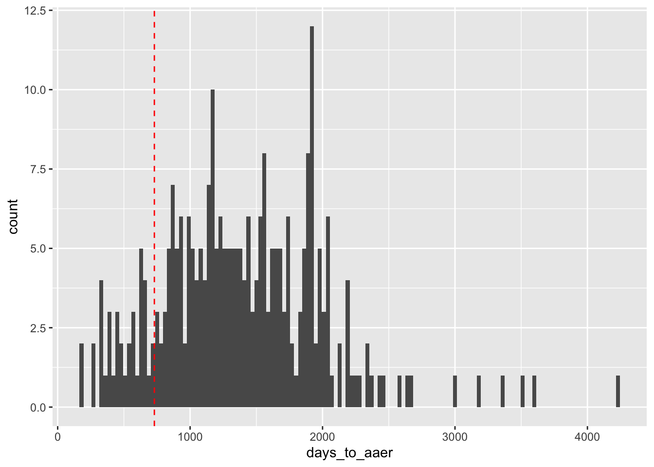

How might we use these data? It would seem appropriate to imagine our analyst looking to apply a model to a fiscal year where that model has been trained on features drawn from prior fiscal years and AAERs revealed to date. For example, if our analyst were now looking to apply a model to data from fiscal 2001, she would be situated somewhere in late 2002 (fiscal 2001 includes firms with fiscal years ending as late as 2002-05-31) and thus would only see AAERs released prior to that time. Assuming the conventional four months for financial data to be released, we might set a “test date” of 2002-09-30 for fiscal 2001, so AAERs with an aaer_date prior to 2002-09-30 would be observable to the analyst.²⁰¹

For concreteness, let’s assume a “test date” of 2002-09-30 and construct a data set of AAERs. In this data set, we measure misstate, which is assumed to be observable to the analyst on test_date, and misstate_latent, which includes accounting fraud observable to the researcher, but not to the analyst.

get_aaers <- function(test_date, include_latent = FALSE) {
  min_aaer_date <- min(aaer_dates$aaer_date, na.rm = TRUE)
  
  df <-
    aaer_dates %>%
    mutate(p_aaer = gsub("^AAER-", "", aaer_num)) %>%
    right_join(aaer_long, by = "p_aaer") %>%
    mutate(aaer_date = coalesce(aaer_date, min_aaer_date)) %>%
    mutate(misstate = aaer_date <= test_date) %>%
    select(gvkey, fyear, misstate)
    
  if (include_latent) {
    df %>% mutate(misstate_latent = TRUE)
  } else {
    df
  }
}

aaers <- get_aaers(test_date = "2002-09-30", include_latent = TRUE)

## Warning in right_join(., aaer_long, by = "p_aaer"): Each row in `x` is expected to match at most 1 row in `y`.
## ℹ Row 21 of `x` matches multiple rows.
## ℹ If multiple matches are expected, set `multiple = "all"` to silence this
##   warning.

Our hypothetical analyst could use misstate from aaers to train a model to predict accounting fraud that, if present, will be revealed at some point in the future. In doing so, our analyst could fit models using data as late as fiscal 2000.²⁰²

Related to this issue, Bao et al. (2020, p. 212) “recode all the fraudulent years in the training period to zero for those cases of serial fraud [accounting fraud spanning multiple consecutive reporting periods] that span both the training and test periods.” Because we require the release of an AAER before coding misstate to one in the training period, and all AAERs are released after any affected fiscal periods (including any that might be considered part of a test period), this kind of recoding is not necessary with our approach.²⁰³

However, just because an analyst could use data from fiscal 2000 doesn’t mean she should. If we accept misstate_latent as “truth”, then misstate can be viewed as measuring true accounting fraud with error.²⁰⁴ Sitting many years in the future (from the perspective of 2001), we can get a handle on the rate of errors assuming a test date at the end of fiscal 2001:

aaers %>% 
  group_by(fyear) %>% 
  summarize(error_rate = mean(misstate != misstate_latent)) %>% 
  filter(fyear <= 2000)

## # A tibble: 11 × 2
##    fyear error_rate
##    <dbl>      <dbl>
##  1  1990     0     
##  2  1991     0     
##  3  1992     0.0741
##  4  1993     0.0333
##  5  1994     0.130 
##  6  1995     0.182 
##  7  1996     0.242 
##  8  1997     0.512 
##  9  1998     0.702 
## 10  1999     0.829 
## 11  2000     0.901

Based on this analysis, it seems plausible that including fiscal 2000 restatements in the data used to train a model for application in fiscal 2001 might increase prediction errors because of the extremely high measurement error in misstate. In fact, the same may even be true of fiscal years 1999 and 1998. Examining this question carefully would require more detailed analysis and we put this analysis outside the scope of this chapter, in part because this analysis could not be conducted by our hypothetical analyst sitting at the end of fiscal 2001, because she would not have access to misstate_latent. Instead, we will table this issue and broadly follow the approach of Bao et al. (2020), who exclude the data on the fiscal year prior to the test year from their training data. That is, for a test year of 2001, we only consider AAERs affecting fiscal 1999 and earlier.²⁰⁵

Before moving on, there is actually one more timing issue to consider. This final issue relates to purpose for which predicting future AAERs is being put. For concreteness, we will consider two possible roles that our hypothetical analyst may have.

The first role is that of a regulator, perhaps even the SEC itself. The SEC might posit that everything that should become an AAER eventually does become an AAER, but yet want to predict future AAERs so as to focus its investigation and enforcement efforts, perhaps to bring AAERs to light sooner rather than later.²⁰⁶ For this purpose, it would seem sensible to want to predict future AAERs whenever they might occur and calibrate models that best serve that end.²⁰⁷

The second role might be that of a short-seller. For example, McCrum (2022) provides numerous examples of short-sellers being interested in information about accounting fraud at Wirecard. One short-seller discussed in McCrum (2022) is Matt Earl, who declared a short position in Wirecard in November 2015 (2022, p. 95), when the stock price was €46.50. Given his short position, Earl might expect to profit if a regulator announced the equivalent of an AAER, as this might be expected to cause the stock price to fall.²⁰⁸ Unfortunately, there was no enforcement release announced by August 2018, when the stock price was at a high of €227.72.²⁰⁹ While Earl’s prediction of accounting fraud was correct, he likely lost a lot of money betting on a stock price fall. By April 2018, Earl was no longer shorting Wirecard (2022, p. 208). What Earl could have profited from was an accurate prediction that Wirecard would be subject to an enforcement action related to accounting fraud in the next $n$ months. Because there was no such action prior to June 2020, his prediction that accounting fraud would be revealed was unprofitable. Of course, a short-seller is not necessarily a passive participant in the flow of information to capital markets and regulators. Earl did produce a report under the name of Zatarra Research and Investigations (2022, p. 100), but was evidently unable to trigger an effective investigation by regulators.²¹⁰

Aside from timing, another set of considerations for our hypothetical users of a prediction model relates to resource constraints and loss functions. A model that predicts “fraud” at hundreds of firm-years only some of which are truly affected by fraud is likely to be difficult for a regulator to act on if there are resource constraints. If a regulator only has the resources to conduct investigations into 10 firms, then it might want a model that assesses the probability of fraud so that it can investigate the 10 firms most likely to be affected. A short-seller is likely constrained by human and capital resources, so may want to identify the firms most likely to be affected so that additional investigation and short-selling can be focused on those firms. These considerations can be incorporated into the objective function used in calibrating the prediction model, as we discuss below.

28.2.3 Merged data

We can now compile our full data set. (Note that we drop misstate_latent, as we would not know that variable when building our model.)

df <-
  aaers %>%
  select(-misstate_latent) %>%
  right_join(features, by = c("gvkey", "fyear")) %>%
  mutate(misstate = coalesce(misstate, FALSE))

We extract the model-building data set (data_train) that we will use in later sections by selecting all observations from df with fiscal years in or before 2001.

data_train <- 
  df %>%
  filter(fyear <= 2001)

28.2.4 Sample splits

In statistical learning, it is common to divide a data set used for developing a statistical prediction model into three disjoint data sets. The first of these is the training data set, which is used to train the model (e.g., estimate coefficients). The second data set is the validation data, which is used to calibrate so-called meta-parameters (discussed below) and choose among alternative modelling approaches. The final data set is the test data which is used to evaluate the performance of the model chosen using the training and validation data sets.

We believe it is helpful to consider the process of training and validating a model as together forming the model-building process and the data set made available to this process as the model-building data.

In principle, if each observation in the data set available to the analyst is independent, these three data sets could be constructed by randomly assigning each observation to one of the data sets.²¹¹

But in the current context, we are simulating a forecasting process, making time an important consideration, as we want to make sure that the process is feasible. For example, it is not realistic to use data from 2008 to train a model that is then tested by “forecasting” a restatement in 1993. Instead, in testing forecasts from a model, it seems more reasonable to require that the model be based on information available at the time the forecast is (hypothetically) being made.

In this regard we follow Bao et al. (2020) in adapting the model-building data set according to the test set and in defining test sets based on fiscal years. Bao et al. (2020) consider a number of test sets and each of these is defined as observations drawn from a single fiscal year (the test year). They then specify the model-building sample for each test state as comprising those firm-year observations occurring in fiscal years at least two years before the test year.

An important point is that the test data set should not be used until the model is finalized. The test data set is meant to be out-of-sample data so as to model the arrival of unseen observations needing classification. If modelling choices are made based on out-of-sample performance, then the test data are no longer truly out of sample and there is a high risk that the performance of the model will be worse when it is confronted with truly novel data.

Having defined the model-building data set, it is necessary to work out how this sample will be split between training and validation data sets. For many models used in statistical learning, there are parameters to be chosen that affect the fitted model, but whose values are not derived directly from the data. These meta-parameters are typically specific to the kind of model under consideration. In penalized logistic regression, there is the penalty parameter $\lambda$. In tree-based models, we might specify a cost parameter or the maximum number of splits.

The validation sample can be used to assess the performance of a candidate modelling approach with different meta-parameter values. The meta-parameter values that maximize performance on the validation sample will be the ones used to create the final model that will be used to predict performance on the test set.

There are different approaches that can be used to create the validation set. Bao et al. (2020) use fiscal 2001 as their validation data set and limit the training data for this purpose to observations with fiscal years between 1991 and 1999.

A more common approach is what is known a $n$-fold cross-validation. With 5-fold cross-validation ($n = 5$), a model-building sample is broken into 5 sub-samples and the model is trained 5 times using 4 sub-samples and evaluated using data on the remaining sub-sample. Values of $n$ commonly used are 5 and 10.

Bao et al. (2020, p. 215) say that “because our fraud data are intertemporal in nature, performing the standard $n$-fold cross validation is inappropriate.” In this regard, Bao et al. (2020) appear to confuse model validation and model testing. It is generally not considered appropriate to test a model using cross-validation, instead cross-validation is used (as the name suggests) for validation.

But Bao et al. (2020) do raise a valid concern with using standard cross-validation due to what they call serial fraud. This issue is probably best understood with an example. Suppose we expanded the feature set to include an indicator for the CFO’s initials being “AF” (perhaps a clue as to “accounting fraud”, but in reality unlikely to mean anything).

aaer_firm_year %>% 
  filter(p_aaer == "1821")

## # A tibble: 1 × 4
##   p_aaer gvkey  min_year max_year
##   <chr>  <chr>     <int>    <int>
## 1 1821   006127     1998     2000

With Enron in the sample for 1998-2000 (when Andrew Fastow was CFO), it’s quite possible that the model would detect the apparent relation between our new feature and accounting fraud and include this in the model. However, this would not improve out-of-sample model performance because Enron would not be in the test sample. So, to maximize out-of-sample performance, we do not want to include this feature in the model and thus want to calibrate a model in a way that discourages the training process from using this feature. If we are not careful in splitting our model-building sample and have Enron in 1998 and 1999 in the training set, and Enron in 2000 in the validation set, then it is going to appear that this feature is helpful and our model will underperform when taken to the test data.

The phenomenon described in the previous paragraph is an instance of overfitting, which refers to the the tendency of models excessively calibrated to fit model-building data to perform poorly when confronted with truly novel data relative to simpler models.²¹²

Therefore in cross-validation, we want to ensure that firm-years for a single AAER are kept in the same sub-sample. In fact, we might want to keep firms in the same cross-validation sub-samples as an extra level of protection against overfitting.²¹³

Another issue related to timing that we might consider in the cross-validation sample is whether it is appropriate to evaluate a model trained on data that includes AAERs at Enron in 1998-2000 in predicting fraud at another firm in, say 1993. We argue the concern about having a feasible forecasting approach that requires us to only forecast future fraud does not preclude training a model using seemingly impossible “prediction” exercises. It is important to recognize that the goals of validating and testing models are very different. In validating the model, we are trying to maximize expected out-of-sample performance (e.g., what it will be when used with a test set), while in testing the model, we are trying to provide a realistic measure of the performance of the model on truly novel data.

Using cross-validation rather than the single fiscal-year validation sample approach used by Bao et al. (2020) offers some benefits, including effectively using the full model-building data set for validation and also validating using data from multiple fiscal years, which reduces the potential for models to be excessively calibrated for models that work well only in fiscal 2001.

To make it easier to implement this for the approaches we discuss below, we first organize our data into folds that can be used below.

n_folds <- 5
folds <- 1:n_folds

sample_splits <- 
  data_train %>%
  select(gvkey) %>%
  distinct() %>%
  mutate(fold = sample(folds, nrow(.), replace = TRUE))

The code above implements the folds for 5-fold cross-validation by assigning each GVKEY to one of 5 folds that will use below. In essence, for fold $i$, we will estimate the model using data in the other folds ($j \neq i$) and then evaluate model performance by comparing the predicted classification for each observation in fold $i$ with its actual classification. We then repeat that for each fold $i$. Later in this chapter, we will also use cross-validation to choose values for meta-parameters.

28.3 Model foundations

There are broadly two basic building blocks with which many statistical learning models are constructed. The first kind of building block fits models using linear combinations of features. For example, in regression-based models, we might use ordinary least squares as the basic unit. With a binary classification problem such as the one we have here, a standard building block is the logistic regression model.

The second kind of building block is the classification tree. We consider each of these building blocks in turn, including their weaknesses, and how these weaknesses can be addressed using approaches that build on them.

28.3.1 Logistic regression

We begin with logistic regression, also known as logit. Logistic regression models the log-odds of an event using a function linear in its parameters:

\[ \log\left(\frac{p}{1-p}\right) = \beta_0 + \beta_1 x_1 + \dots + \beta_P x_P.\] Here $p$ is the modelled probability of the event’s occurrence and $P$ denotes the number of predictors. Kuhn and Johnson (2013, p. 280) suggest that “the logistic regression model is very popular due to its simplicity and ability to make inferential statements about model terms.” While logit can be shown to be the maximum likelihood estimator for certain structural models, it is not always optimized for prediction problems (see Kuhn and Johnson, 2013, p. 281). While we will not use logit to “make inferential statements” in this chapter, we explore it given its popularity and simplicity.

Having identified a model-building data set, we first fit a logistic regression model and store the result in fm1. Like ordinary least-squares (OLS) regression, logit falls in the class of models known as generalized linear models (GLMs), and thus can be easily estimated using the glm function provided with Base R. All we need to do is specify family = binomial and the glm function will choose logit as the link function (link = "logit" is the default for the binomial family).

formula <- paste(y_var, "~", paste(X_vars, collapse = " + "))
fm1 <- glm(formula, data = data_train, family = binomial)

We can assess within-sample performance of the logit model by comparing the predicted outcomes with the actual outcomes for data_train. Here we use the fitted probability (prob) to assign the predicted classification as TRUE when prob > 0.5 and FALSE otherwise. (As discussed below, there may be reasons to choose a different cut-off from 0.5.)

within_sample <-
  data_train %>%
  mutate(score = predict(fm1, newdata = ., type = "response"),
         predicted = as.integer(score > 0.5))

We can produce a confusion matrix, which is a tabulation of number of observations in the sample by predicted and true outcome values.

table(predicted = within_sample$predicted, 
      response = within_sample$misstate)

##          response
## predicted FALSE  TRUE
##         0 66967   208
##         1     0     1

Here we see 1 true positive cases, 66967 true negative cases, 208 false negative cases, and 0 false positive cases.

While there are no meta-parameters to select with the basic logistic regression model, we can use cross-validation as an approach for estimating out-of-sample prediction performance.

The following function takes the argument fold, fits a logit model for observations not in that fold, then classifies observations that are in that fold, and returns the values.

logit_predict <- function(fold) {
  dft <-
    data_train %>%
    inner_join(sample_splits, by = "gvkey")
  
  fm1 <-
    dft %>%
    filter(fold != !!fold) %>%
    glm(formula, data = ., family = binomial)
  
  dft %>%
    filter(fold == !!fold) %>%
    mutate(score = predict(fm1, newdata = ., type = "response"),
           predicted = as.integer(score > 0.5)) %>%
    select(gvkey, fyear, score, predicted)
}

We can call logit_predict for each fold, combine the results into a single data frame, and then join with data on misstate from data_train.

logit_fit <- 
  bind_rows(lapply(folds, logit_predict)) %>%
  inner_join(data_train, by = c("gvkey", "fyear")) %>% 
  select(gvkey, fyear, predicted, score, misstate)

The predicted value for each observation is based on a model that was trained using data excluding the firm for which we are predicting.

head(logit_fit)

## # A tibble: 6 × 5
##   gvkey  fyear predicted   score misstate
##   <chr>  <dbl>     <int>   <dbl> <lgl>   
## 1 111534  1998         0 0.00326 TRUE    
## 2 111534  1999         0 0.0129  TRUE    
## 3 028354  1993         0 0.00284 TRUE    
## 4 013070  1994         0 0.00266 TRUE    
## 5 013070  1995         0 0.00315 TRUE    
## 6 013070  1996         0 0.00275 TRUE

Again we can produce the confusion matrix using the predictions from cross-validation. Now we see 0 true positive cases, 66953 true negative cases, 209 false negative cases, and 18 false positive cases.

table(predicted = logit_fit$predicted, response = logit_fit$misstate)

##          response
## predicted FALSE  TRUE
##         0 66953   209
##         1    18     0

As poor as within-sample classification performance was, it seems it was actually optimistic relative to performance assessed using cross-validation.

28.3.2 Classification trees

The second fundamental building block that we consider here is the classification tree. According to Kuhn and Johnson (2013, p. 173), “tree-based models consist of one or more nested if-then statements for the predictors that partition the data. Within these partitions, a model is used to predict the outcome.” The models are often called simply trees for reasons that are clear from their typical graphical representation (see below). Other terminology follows from the tree metaphor: the splits give rise the branches and a terminal node of a tree is called a leaf.²¹⁴

Trees can be categorized as either regression trees or as classification trees. A typical output for a regression tree is a predicted numerical value for given values of covariates. In contrast, a typical output for a classification tree is a predicted class value (e.g., “hot dog” or “not hot dog”). Given our focus on binary classification problems, we focus on classification trees.

There are many approaches for building trees. One of the oldest and most popular techniques is the classification and regression tree (CART) of Breiman et al. (1984). The CART algorithm is a form of recursive partitioning, where the partitioning refers to the division of the sample into disjoint sets and recursive refers to the fact that the partitioning can be performed recursively (i.e., each set formed by partition can be partitioned in turn).

Algorithms for fitting CART models are provided by the rpart function offered by the rpart package. We now fit a model (fm2) using recursive partitioning. We set two control parameters: cp and minbucket.²¹⁵

fm2 <- rpart(formula, data = data_train, 
             control = rpart.control(cp = 0.001, minbucket = 5), method = "class")

While the logistic regression model stored in fm1 is described by coefficients on each of the 28 features, the tree stored in fm2 can be represented by the graph depicted below. Because we are using the built-in plot method for fm2, we use the par function to set the parameter cex, which controls the size of text displayed on the plot, and we use the text function to add text to the plot.

par(cex = 0.5)
plot(fm2)
text(fm2)

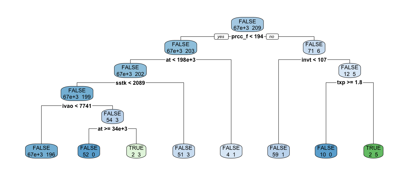
Again we can assess within-sample performance. Note that we need slightly different commands to extract predicted probabilities and classes from fm2 from those we used with fm1.

within_sample <-
  data_train %>%
  mutate(prob = predict(fm2, newdata = .)[, 2],
         predicted = prob > 0.5)

table(predicted = within_sample$predicted, 
      response = within_sample$misstate)

##          response
## predicted FALSE  TRUE
##     FALSE 66963   201
##     TRUE      4     8

Here we see 8 true positive cases, 66963 true negative cases, 201 false negative cases, and 4 false positive cases.

28.3.3 Exercises

One claimed benefit of classification trees is their ease of interpretation. Can you provide an intuitive explanation for the fitted tree above? If so, outline your explanation. If not, what challenges prevent you from doing so?
Use 5-fold cross validation to assess the performance of the classification tree approach using the parameters above.
What do the parameters cp and minbucket represent?
How does the classification tree change if you increase the parameter cp?
Use 5-fold cross validation to assess the performance of the classification tree approach with three different parameters for minbucket (the one used above and two others).

28.4 Performance metrics

It is intuitively clear that the performance of the models is not particularly impressive, but in general we need ways to measure model performance more formally and precisely. A number of evaluation metrics are available to measure the performance of prediction models. In this section, we discuss some of these metrics with a focus on two-class classification problems.²¹⁶

28.4.1 Accuracy

One standard classification performance metric is accuracy, defined as $\frac{TP+TN}{TP+FN+FP+TN}$, where $TP$ (true positive) is (in our current context) the number of fraudulent firm-years that are correctly classified as fraud; $FN$ (false negative) is the number of fraudulent firm-years that are misclassified as non-fraud; $TN$ (true negative) is the number of non-fraudulent firm-years that are correctly classified as non-fraud; and $FP$ (false positive) is the number of non-fraudulent firm-years that are misclassified as fraud.

Unfortunately, accuracy is a not a very useful metric in this setting because of the severe class imbalance. With fewer than 1% of firms in a typical year being affected by accounting fraud, simply classifying all firm-years as non-fraud would have accuracy of more than 99%.

Two other statistics that are often considered are sensitivity (also known as the true positive rate, or TPR) and specificity (also known as the **true negative rate* or TNR)

\[ \textit{Sensitivity} = \textit{TPR} = \frac{TP}{TP + FN} \]

\[ \textit{Specificity} = \textit{TNR} = \frac{TN}{TN + FP} \] Often we focus on the complement to specificity, which is know as the false positive rate (FPR) and calculated as follows:

\[ 1 - \textit{Specificity} = \textit{FPR} = 1 - \frac{TN}{TN + FP}= \frac{FP}{TN + FP}\]

28.4.2 AUC

There is an inherent trade-off between sensitivity and specificity. A classification model will typically return something like an estimated probability that an observation is a positive case. We can choose a cut-off probability and classify all observations with an estimated probability at or above the cut-off as a positive case, and classify all observations with estimated probabilities below the cut-off as negative cases. Starting at a cut-off of zero, every observation would be classified as a positive and the TPR would be 1, but the FPR would also be 1. As the cut-off increases, both the TPR and the FPR will decrease.

If we collect the pairs of values of TPR and FPR as we increase the cut-off, we can plot the TPR against the FPR to form what is called the response operator curve (or ROC).

In terms of the ROC, the worst-case model just randomly assigns probabilities to each observation. So with a cut-off of 0.25, we’d classify 75% of observations as positive and 25% as negative. In expectation, we’d have 75% of the positive cases classified as positive, and 75% of the negative cases classified as positive, so the TPR and FPR values would be equal in expectation. This would yield an ROC close to the 45-degree line.

The best-case model would be a perfect classifier that yielded zero FNR and 100% TPR. This would yield an ROC that rose vertically along the $y$-axis and horizontally at $y = 100\%$.

This suggests the area under the ROC curve (or AUC) as a measure of the quality of a model, with values of $0.5$ for the random-guess model and $1$ for the perfect classifier. Below, we follow Bao et al. (2020) (and many others) in using AUC as the performance measure we use to evaluate models.

28.4.3 NDCG@k

Bao et al. (2020) also consider an alternative performance evaluation metric called the normalized discounted cumulative gain at position $k$ (NDCG@k).

NDCG@k metric can be motivated using the idea of budget constraints. Suppose that a regulator (or other party interesting in unearthing frauds) has a limited budget and can only investigate $k$ frauds in a given year. Denoting the number of actual frauds in a year as $j$, if $j \geq k$, then the best that the regulator can do is to investigate $k$ cases, all of which are frauds. If $j < k$, then the regulator can do no better than investigating $k$ cases with all $j$ frauds being among those investigated.

The assumption is that the regulator investigates the $k$ cases with the highest estimated probability of being frauds (scores). This suggests a performance measure that scores a model higher the greater the number of true frauds ranked in the top $k$ scores.

The measure NDCG@k is such a measure. NDCG@k also awards more “points” the higher in the list (based on scores) each true fraud is placed. This is implemented by multiplying each correct guess by $1/\log_2 (i + 1)$. Formally, the discounted cumulative gain at position $k$ is defined as follows: \[ \textrm{DCG@k} = \sum_{i=1}^k \textit{rel}_i/\log_2 (i + 1) \]

The measure NDCG@k is DCG@k normalized by the the DCG@k value obtained when all the true instances of fraud are ranked at the top of the ranking list. Hence, the values of NDCG@k are bounded between $0$ and $1$, and a higher value represents better performance.

Bao et al. (2020) select $k$ so that the number of firm-years in the ranking list represents 1% of all the firm-years in a test year. Bao et al. (2020) “select a cut-off of 1% because the average frequency of accounting fraud punished by the SEC’s AAERs is typically less than 1% of all firms in a year.”

Bao et al. (2020) report modified versions of sensitivity and specificity: $\text{Sensitivity@k} = \frac{TP@k}{TP@k + FN@k}$ and $\text{Precision@k} = \frac{TP@k}{TP@k + FP@k}$ where TP@k, FN@k and FP@k are analogous to TP, FN and FP, but based on classifying as frauds only the $k\%$ of observations with the highest scores.

28.5 Penalized models

Having a number of ways to measure model performance alone does not address the basic problem of poor model performance using the two fundamental approaches above. In this section and the next, we describe two strategies that can be used to improve model performance.

The first approach uses penalized models. Perhaps the easiest way to understand penalized models is to recognize that many common modelling approaches seek to minimize the sum of squared errors

\[ \textrm{SSE} = \sum_{i = 1}^{n} (y_i - \hat{y}_i )^2. \]

With penalized models, the objective is modified by adding a penalty term. For example, in ridge regression the following objective function is minimized.²¹⁷:

\[ \textrm{SSE}_{L_2} = \sum_{i = 1}^{n} (y_i - \hat{y}_i )^2 + \lambda \sum_{j=1}^{P} \beta_j^2. \] An alternative approach is least absolute shrinkage and selection operator (or lasso) model, which uses the following objective function:

\[ \textrm{SSE}_{L_1} = \sum_{i = 1}^{n} (y_i - \hat{y}_i )^2 + \lambda \sum_{j=1}^{P} \left|\beta_j \right|.\] While both ridge regression and lasso will shrink coefficients towards zero (hence the alternative term shrinkage methods), some coefficients will be set to zero by lasso for some value of $\lambda$. In effect, lasso performs both shrinkage and feature selection.

A third shrinkage method worth mentioning is elastic net (Kuhn and Johnson, 2013, p. 126), which includes the penalties from both ridge regression and lasso

\[ \textrm{SSE}_{\textrm{ENet}} = \sum_{i = 1}^{n} (y_i - \hat{y}_i )^2 + \lambda_1 \sum_{j=1}^{P} \beta_j^2 + \lambda_2 \sum_{j=1}^{P} \left|\beta_j \right|.\] One aspect of these penalized objective functions that we have not discussed is $\lambda$. Implicitly, $\lambda > 0$ (if $\lambda = 0$, then the penalty term is zero), but we have said nothing about how this parameter is selected.²¹⁸ Instead, $\lambda$ is a meta-parameter of the kind alluded to above, as it is not estimated directly as part of the estimation process.

A common approach to setting meta-parameters like $\lambda$ is cross-validation. With cross-validation, a number of candidate values of $\lambda$ are considered. For each candidate value and each cross-validation fold, the model is estimated omitting the data in the fold. The performance of the model is evaluated using predicted values for the cross-validation folds (e.g., the average mean-squared error, or MSE, across all folds). Finally, the value $\lambda$ that maximizes performance (e.g., minimizes MSE) is chosen as the value to be used when applying the model to new data (e.g., test data when applicable).

To illustrate, we use the lasso analogue to the logit regression we estimated above.²¹⁹ For this purpose, we use the glmnet library and specify alpha = 1 to focus on the lasso model.

The glmnet library contains built-in functionality for cross-validation. We simply need to specify the performance metric to use in evaluating models (here we set type.measure = "auc" to use AUC) and—because we constructed our folds to put all observations on a given firm in the same fold—the foldid for each observation

dft <-
  data_train %>%
  inner_join(sample_splits, by = "gvkey")

fm_lasso_cv <-
  cv.glmnet(x = as.matrix(dft[X_vars]),
            y = dft[[y_var]],
            family = "binomial",
            alpha = 1,
            type.measure = "auc",
            foldid = dft[["fold"]],
            keep = TRUE)

The glmnet function will automatically consider a range of $\lambda$ values. Note that the scale of the features matters with penalized regression, as the penalties increase with the magnitude of the coefficients, which in turn depends on the scale of the variables. For example, a logit coefficient on at expressed in millions of dollars of $0.123$ is equivalent to a coefficient of $123$ on at expressed in thousands of dollars. Thus glmnet will by default scale the features (see ? glmnet for additional details).

tibble(lambda = fm_lasso_cv$lambda, auc = fm_lasso_cv$cvm) %>% 
  ggplot(aes(x = lambda, y = auc)) +
  geom_line()

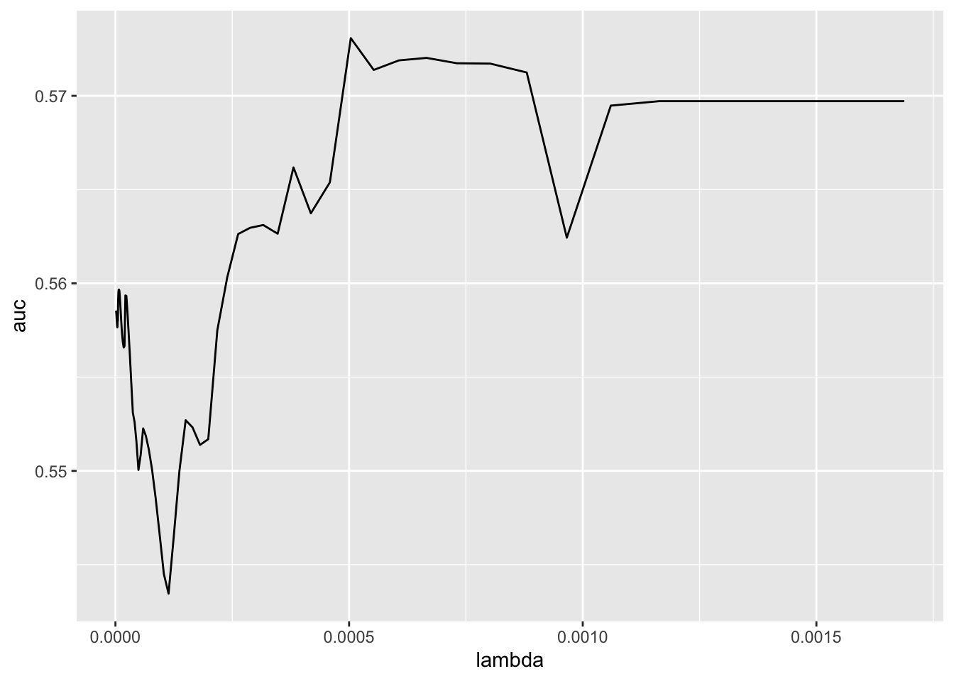
Here we see that AUC is maximized with $\lambda \approx 1.2e-05$.

Predicted values for each value of $\lambda$ considered are stored in fit.preval of fm_lasso_cv as log-odds ratios. We can convert these to probabilities using the function $f(x) = \frac{\exp(x)}{1+\exp(x)}$. Here we select the value of $\lambda$ that maximizes AUC (this is stored in fm_lasso_cv$lambda.min).²²⁰

idmin <- match(fm_lasso_cv$lambda.min, fm_lasso_cv$lambda)

fit_lasso_cv <- 
  dft %>%
  select(misstate) %>%
  mutate(logodds = fm_lasso_cv$fit.preval[, idmin],
         prob = exp(logodds)/(1 + exp(logodds)),
         predicted = logodds > 0)

From this we can calculate the confusion matrix based on the models fitted using cross-validation.

table(predicted = fit_lasso_cv$predicted, 
      response = fit_lasso_cv$misstate)

##          response
## predicted FALSE  TRUE
##     FALSE 66956   209
##     TRUE     11     0

We can produce the fitted model based on our chosen $\lambda$ by estimating a single model for the entire training data set. We store this model in fm_lasso.

fm_lasso <- glmnet(x = as.matrix(data_train[X_vars]), 
                   y = data_train[[y_var]],
                   family = "binomial",
                   lambda = fm_lasso_cv$lambda.min,
                   alpha = 1)

28.5.1 Discussion questions and exercises

What features are selected by the lasso model in this case? (Hint: You may find it useful to inspect fm_lasso$beta[, 1].)
Modify the code above to estimate a ridge regression model. (Hint: Set alpha = 0.)
Describe how would you estimate an elastic net model. (Hint: Discussion here might be useful. One approach would be to put some of the steps above in a function that accepts alpha as an argument and then estimate over different values of $\alpha$.)
Calculate AUC and produce the confusion matrix for fm_lasso applied to data_train (i.e., in sample). Interpret these results. (Hint: You might use this code: predict(fm_lasso, newx = as.matrix(data_train[X_vars])) and the auc function supplied with the farr package.)
Calculate the AUC for the data stored in within_sample above (this is for the tree stored in fm2).

28.6 Ensemble methods

A second approach to addressing the weaknesses of building models directly from the building blocks uses ensemble methods, which are methods that combine the predictions from many models to generate a single prediction for each observation. The ensemble methods we cover here are all based on trees.

One of the earliest ensemble methods is bagging, which is short for bootstrap aggregation. With bagging a value $M$ is selected and for each $i \in (1, \dots, M)$ a bootstrap sample of the original data is taken and a model is fit. The prediction for any observation is an average of the predictions of the $M$ models.²²¹

One benefit of bagging is that for any given observation, several of the $M$ models will not have used that observation in the fitting process, so the predictions from these models are, in a sense, out of sample for that observation. Such observations are termed out-of-bag and provide a natural measure of the predictive performance much like cross-validation measures.

One additional aspect of bagging is that there are no dependencies between the fitted models. So one could in principle divide the estimation of the $M$ models between $M$ computers (or cores) and (assuming sufficient computing resources) generate a prediction almost as quickly as one could from a single model.

A refinement of bagging is random forests, which not only uses bootstrap samples of the observations, but also randomly draws a subset of $k < P$ features in fitting each model. By randomly selecting features in addition to randomly selecting observations, random forests generate trees with lower correlation than bagging does. This can reduce the risk that the model overfits the sample using certain features and also produces more robust models when features are highly correlated.

The final set of ensemble methods we discuss are known as boosting methods. The basic idea of boosting is that each observation has a weight that varies from one iteration to the next: observations that are incorrectly classified in iteration $k$ receive more weight in iteration $k + 1$. In this way, the observations that are difficult to classify can receive increasingly larger weight until the algorithm is able to identify a model that classifies them correctly. Below we describe two boosting algorithms in more detail: AdaBoost—which was “the first practical implementation of boosting theory” (Kuhn and Johnson, 2013, p. 389)—and RUSBoost—which was introduced to accounting research by Bao et al. (2020).²²² Because the outcome of iteration $k$ affects the model fit in iteration $k + 1$, boosting is not as easily implemented in parallel as bagging or random forests.

28.6.1 AdaBoost

Boosting is perhaps best understood in the context of an actual algorithm implementing it. Hastie et al. (2013) outline the AdaBoost algorithm as follows:

Initialize the observation weights $w_i = \frac{1}{N}$, $i = 1,2,\dots,N$.
For $m = 1 \to M$:
1. Fit a classifier $G_m(x)$ to the training data using weights $w_i$.
2. Compute \[ \mathrm{err}_m = \frac{\sum_{i=1}^N w_i I(y_i \neq G_m(x_i))}{\sum_{i=1}^{N} w_i}\]
3. Compute $\alpha_m = \log((1 - \mathrm{err}_m)/\mathrm{err})$.
4. Set $w_i \leftarrow w_i \exp\left[\alpha_m I(y_i \neq G_m(x_i)) \right]$.
Output $G(x) = \mathrm{sign} \left[\sum_{m=1}^M \alpha_m G_m (x) \right]$

A couple of observations on this algorithm are in order. First, step 3 implicitly assumes that the classes are coded as either $+1$ or $-1$ so that the sign indicates the class. Second, we have not described what classifier is represented by $G_m(x)$.

We provide an implementation of AdaBoost in the farr package. Because the RUSBoost algorithm we discuss below is a variation on AdaBoost, we use one function (rusboost) to cover both AdaBoost (rus = FALSE) and RUSBoost (rus = TRUE). We use the rpart function discussed above as the basic building block for rusboost (i.e., $G_m(x)$). This means any arguments that can be passed to rpart via the control argument can be used with rusboost.

In addition, a user of rusboost can specify the number of iterations ($M$) using the size argument and a learning rate ($L \in (0, 1]$) using the learn_rate argument. The learning rate modifies step 2(c) of the AdaBoost algorithm above to:

Compute $\alpha_m = L \log((1 - \mathrm{err}_m)/\mathrm{err})$.

(Hence the default learn_rate = 1 implements the algorithm above.)

We make a convenience function fit_rus_model that allows us to set maxdepth and minbucket values passed to rpart directly.

fit_rus_model <- function(df, size = 30, rus = TRUE, learn_rate = 1,
                          maxdepth = NULL, minbucket = NULL,
                          ir = 1) {
  if (!is.null(maxdepth)) control <- rpart.control(maxdepth = maxdepth) 
  if (!is.null(minbucket)) control <- rpart.control(minbucket = minbucket)
  
  fm <- rusboost(formula, df, size = size, ir = ir, learn_rate = learn_rate, rus = rus,
                 control = control)
  return(fm)
}

We next create a convenience function for calculating fitted probabilities and predicted classes for data in a fold.

rus_predict <- function(fold, ...) {
  dft <-
    data_train %>%
    inner_join(sample_splits, by = "gvkey") %>%
    mutate(misstate = as.integer(misstate))
  
  fm <-
    dft %>%
    filter(fold != !!fold) %>%
    fit_rus_model(...)
  
  res <-
    dft %>%
    filter(fold == !!fold) %>% 
    mutate(prob = predict(fm, ., type = "prob"),
           predicted = predict(fm, ., type = "class")) %>%
    select(gvkey, fyear, prob, predicted)
  
  res
}

We next create a function that fits models by fold and returns the resulting cross-validated AUC. Note that we use mclapply from the parallel library here; this may not work on Windows (if so, replace mclapply with lapply and delete mc.cores = 8).

get_auc <- function(...) {
  set.seed(2021)
  rus_fit <- 
    bind_rows(mclapply(folds, rus_predict, mc.cores = 8, ...)) %>%
    inner_join(data_train, by = c("gvkey", "fyear")) %>% 
    select(gvkey, fyear, predicted, prob, misstate)
  
  auc(score = rus_fit$prob, response = as.integer(rus_fit$misstate))
}

The meta-parameters that we evaluated as size ($M$, the number of iterations), learn_rate ($L$, the learning rate), and maxdepth (the maximum depth of trees).

params <- expand_grid(size = c(30, 50),
                      learn_rate = c(0.1, 0.5, 1),
                      maxdepth = c(3, 5, 7))

We can now use our get_auc function to evaluate the model performance for each of the possible parameter values in params.

adaboost_results <-
  params %>% 
  mutate(auc = unlist(Map(get_auc, 
                          rus = FALSE,
                          size = size, 
                          learn_rate = learn_rate, 
                          maxdepth = maxdepth)))

## Warning: There were 18 warnings in `mutate()`.
## The first warning was:
## ℹ In argument: `auc = unlist(...)`.
## Caused by warning in `inner_join()`:
## ! Each row in `x` is expected to match at most 1 row in `y`.
## ℹ Row 58 of `x` matches multiple rows.
## ℹ If multiple matches are expected, set `multiple = "all"` to silence this
##   warning.
## ℹ Run `dplyr::last_dplyr_warnings()` to see the 17 remaining warnings.

Here are the first few rows of the results.

adaboost_results %>%
  arrange(desc(auc)) %>%
  head() %>%
  knitr::kable()

size	learn_rate	maxdepth	auc
30	0.1	7	0.6662838
50	0.1	7	0.6503775
50	0.1	5	0.6447974
30	0.1	5	0.6424609
50	0.5	7	0.6415961
50	0.1	3	0.6267669

We store the row (set of parameter values) that maximizes AUC in optim_ada.

optim_ada <- adaboost_results %>% filter(auc == max(auc))

28.6.2 RUSBoost

RUSBoost is a variant of AdaBoost that makes use of random undersampling (RUS) to address the problem of class imbalance learning (Seiffert et al., 2008). When there are very few positive cases (i.e., fraud firm-years) relative to negative cases, RUSBoost allows a model to train using samples with substantially more positive cases than found in the broader population. Given the relatively small number of fraud firm-years, the setting of Bao et al. (2020) seems to be a good one for RUSBoost. Seiffert et al. (2008) lay out the RUSBoost algorithm as follows:²²³

Initialize the observation weights $w_i = \frac{1}{N}$, $i = 1,2,\dots, N$.
For $m = 1 \to M$:
1. Create temporary training dataset $S^{'}_t$ with distribution $D^{'}_t$ using random under-sampling
2. Fit a classifier $G_m(x)$ to the training data using weights $w_i$.
3. Compute \[ \mathrm{err}_m = \frac{\sum_{i=1}^N w_i I(y_i \neq G_m(x_i))}{\sum_{i=1}^{N} w_i}\]
4. Compute $\alpha_m = L \log((1 - \mathrm{err}_m)/\mathrm{err})$.
5. Set $w_i \leftarrow w_i \exp\left[\alpha_m I(y_i \neq G_m(x_i)) \right]$.
Output $G(x) = \mathrm{sign} \left[\sum_{m=1}^M \alpha_m G_m (x) \right]$

In each iteration, the RUS algorithm samples from the training data differently for fraudulent and non-fraudulent firm-years. RUSBoost requires setting the ratio between the number of undersampled majority class observations (i.e., non-fraud) and the number of minority class observations (i.e., fraud). The rusboost function allows the user to specify this ratio using the ir argument. Bao et al. (2020) estimate RUSBoost models using a 1:1 ratio (i.e., ir = 1), which means each sample they used in estimation contained the same number of fraud and non-fraudulent observations.

Fraudulent firm-years—which are much rarer—are randomly sampled with replacement up to their number in the training sample (e.g., if there are 25 fraudulent observations in the training data, 25 such observations will be in the training sample used). Non-fraudulent firm-years—which are more numerous—are randomly sampled without replacement up to a number that is typically expressed as a multiple of the number of fraudulent observations in the training sample (e.g., if there are 25 fraudulent observations in the training data and ir = 1, 25 such observations will be in the training sample used).

In addition to ir = 1, we consider ir = 2 (the latter selecting two non-fraud observations for each fraud observation).

We use a different set of meta-parameter values for size, learn_rate, and maxdepth for RUSBoost than we did for AdaBoost, as the relation between meta-parameters and performance differs.²²⁴

params_rus <- expand_grid(size = c(30, 100, 200, 300),
                      learn_rate = c(0.01, 0.1, 0.5, 1),
                      maxdepth = c(2, 3, 5, 10, 15),
                      ir = c(1, 2))

Again, we can now use the get_auc function to evaluate the model performance for each of the possible parameter values (now in params_rus).

rusboost_results <-
  params_rus %>% 
  mutate(auc = unlist(Map(get_auc, 
                          rus = TRUE,
                          size = size, 
                          learn_rate = learn_rate, 
                          maxdepth = maxdepth,
                          ir = ir)))

## Warning: There were 160 warnings in `mutate()`.
## The first warning was:
## ℹ In argument: `auc = unlist(...)`.
## Caused by warning in `inner_join()`:
## ! Each row in `x` is expected to match at most 1 row in `y`.
## ℹ Row 58 of `x` matches multiple rows.
## ℹ If multiple matches are expected, set `multiple = "all"` to silence this
##   warning.
## ℹ Run `dplyr::last_dplyr_warnings()` to see the 159 remaining warnings.

Here are the first few rows of the results.

rusboost_results %>%
  arrange(desc(auc)) %>%
  head() %>%
  knitr::kable()

size	learn_rate	maxdepth	ir	auc
30	0.01	10	2	0.6943248
300	0.01	15	2	0.6894045
200	0.01	10	2	0.6879628
300	0.01	10	2	0.6867877
200	0.01	15	2	0.6865816
200	0.10	15	1	0.6853092

We store the row that maximizes AUC in optim_rus

optim_rus <- rusboost_results %>% filter(auc == max(auc))

Compared with AdaBoost, we see that RUSBoost performance is maximized with larger models (size is 30 rather than 30), deeper trees (maxdepth is 10 rather than 7). We see that both models use a learn_rate less than 1.

Before testing our models, it is noteworthy that the AUCs for both AdaBoost and RUSBoost are appreciably higher than those for the logit model, the single tree, and the penalized logit models from above.

28.6.3 Discussion questions

Provide reasons why the tree-based models outperform the logit-based models in this setting? Do you think this might be related to the set of features considered? How might you alter the features if you wanted to improve the performance of the logit-based models?

28.7 Testing models

We now consider the out-of-sample performance of our models. Given the apparent superiority of the boosted ensemble approaches (AdaBoost and RUSBoost) over the other approaches, we focus on those two approaches here.

We follow Bao et al. (2020) in a number of respects. First, we use fiscal years 2003 through 2008 as our test years. Second, we fit a separate model for each test year using data on AAERs that had been released on the posited test date for each test year.

Third, we exclude the year prior to the test year from the model-fitting data set (we do this by using filter(fyear <= test_year - gap) where gap = 2). But note that the rationale provided by Bao et al. (2020) for omitting this year differs from ours: Bao et al. (2020) wanted some assurance that the AAERs were observable when building the test model; in contrast, we simply want to reduce measurement error in the misstate variable when using too-recent a sample.²²⁵

Fourth, rather that using gap to get assurance that the AAERs were observable when building the test model, we use data on AAER dates to ensure that the AAERs we use had been revealed by our test dates. For each test_year, we assume that we are fitting a model on 30 September in the year after test_year, so as to allow at least four months for financial statement data to be disclosed (fiscal years for, say, 2001 can end as late as 31 May 2002, so 30 September gives four months for these).

test_years <- 2003:2008

test_dates <- 
  tibble(test_year = test_years) %>%
  mutate(test_date = as.Date(paste0(test_year + 1, "-09-30")))

We now create a function that allows us to pass a set of features, specify the test_year and the parameters to be used in fitting the model (e.g., learn_rate and ir) and which returns a fitted model.

train_model <- function(features, test_year, gap = 2,
                        size, rus = TRUE, learn_rate, ir, control) {
  
  test_date <- 
    test_dates %>% 
    filter(test_year == !!test_year) %>%
    select(test_date) %>%
    pull()
  
  aaers <- get_aaers(test_date = test_date)

  data_train <- 
    aaers %>%
    right_join(features, by = c("gvkey", "fyear")) %>%
    filter(fyear <= test_year - gap) %>%
    mutate(misstate = as.integer(coalesce(misstate, FALSE)))
  
  fm <- rusboost(formula, data_train, size = size, learn_rate = learn_rate, 
                 rus = rus, ir = ir, control = control)
  return(fm)
}

Note that in training our final model, we can use all available data in the training data set. For a test year of 2003, our training data set is the same as that used for selecting the meta-parameters above, but there we generally only used a subset of the data (i.e., in cross-validation) in fitting models in that process.

We next create a function that allows us to pass a set of features (features), a fitted model (fm) and to specify the test year (test_year) and which returns the predicted values and estimated probabilities for the test observations.

test_model <- function(features, fm, test_year) {
  
  target <- as.character(stats::as.formula(fm[["formula"]])[[2]])
  
  df <- 
    features %>%
    left_join(aaer_long, by = c("gvkey", "fyear")) %>%
    select(-max_year, -min_year) %>%
    mutate(misstate = as.integer(!is.na(p_aaer)))

  data_test <- 
    df %>%
    filter(fyear == test_year)

  return(list(score = predict(fm, data_test, type = "prob"),
              predicted = as.integer(predict(fm, data_test, 
                                             type = "class") == 1), 
              response = as.integer(data_test[[target]] == 1)))
}

We next make a convenience function that calls train_model then test_model in turn.²²⁶

fit_test <- function(x, features, gap = 2,
                     size, rus = TRUE, learn_rate, ir = 1, control) {
  set.seed(2021)
  fm <- train_model(features = features, test_year = x, 
                    size = size, rus = rus, ir = ir,
                    learn_rate = learn_rate, control = control, gap = gap)
  test_model(features = features, fm = fm, test_year = x)
}

We first test AdaBoost using the meta-parameter values stored in optim_ada and store the results in results_ada. We have included the values generated from code in Section 28.6 above here so that you do not need to run the code from that section.

optim_ada <- tibble(size = 30, learn_rate = 0.1, maxdepth = 7)

Again, we use mclapply from the parallel library here; this may not work on Windows (if so, replace mclapply with lapply and delete mc.cores = 8).

results_ada <- mclapply(test_years, fit_test, 
                        features = features, 
                        size = optim_ada$size,
                        rus = FALSE, 
                        learn_rate = optim_ada$learn_rate,
                        control = rpart.control(
                        maxdepth = optim_ada$maxdepth),
                        mc.cores = 8)

We then test RUSBoost using the meta-parameter values stored in optim_rus and store the results in results_rus. We have included the values generated from code in Section 28.6 above here so that you do not need to run the code from that section.

optim_rus <- tibble(size = 30, learn_rate = 0.01, maxdepth = 10, ir = 2)

results_rus <- mclapply(test_years, fit_test, 
                        features = features, 
                        size = optim_rus$size,
                        rus = TRUE,
                        ir = optim_rus$ir, 
                        learn_rate = optim_rus$learn_rate,
                        control = rpart.control(
                          maxdepth = optim_rus$maxdepth),
                        mc.cores = 8)

To make it easier to tabulate results, we create a small function that collects performance statistics for a set of results that can be used to tabulate the results.

get_stats <- function(results) {
  response <- results$response
  score <- results$score
  
  ndcg_k <- function(k) {
    c(ndcg(score, response, k = k))
  }
  
  res <- list(auc(score, response),
              unlist(lapply(seq(0.01, 0.03, 0.01), ndcg_k)))
  unlist(res)
}

The analyses in Bao et al. (2020) appear to evaluate test performance using the means across test years, so we make a small function (add_means) to add a row of means to the bottom of a data frame and use this function in table_results, which is a function that extracts performance statistics from a set of results, adds means, then formats the resulting data frame for display.

add_means <- function(df) {
  bind_rows(df, summarize_all(df, mean))
}

table_results <- function(results, ...) {
  results %>% 
  lapply(get_stats) %>%
  bind_rows() %>%
  add_means() %>%
  mutate(test_year = c(test_years, "Mean")) %>% 
  select(test_year, everything()) %>%
  knitr::kable(digits = 4, ...)
}

We can now simply call table_results for results_ada and results_rus in turn.

table_results(results_ada)

test_year	auc	ndcg_0.01	ndcg_0.02	ndcg_0.03
2003	0.7010	0.0451	0.0504	0.0760
2004	0.6292	0.0257	0.0361	0.0458
2005	0.6821	0.0182	0.0182	0.0413
2006	0.6851	0.0000	0.0308	0.0308
2007	0.5674	0.0000	0.0000	0.0148
2008	0.6061	0.0000	0.0180	0.0180
Mean	0.6452	0.0148	0.0256	0.0378

table_results(results_rus)

test_year	auc	ndcg_0.01	ndcg_0.02	ndcg_0.03
2003	0.7134	0.1116	0.1300	0.1385
2004	0.7048	0.0321	0.0321	0.0321
2005	0.7019	0.0359	0.0359	0.0478
2006	0.7237	0.0181	0.0344	0.0492
2007	0.5636	0.0000	0.0000	0.0000
2008	0.6140	0.0234	0.0234	0.0234
Mean	0.6702	0.0368	0.0426	0.0485

From the results above, it does seem that RUSBoost is superior to AdaBoost in this current setting using the features drawn from Bao et al. (2020). Note that Bao et al. (2020) do not separately consider AdaBoost as an alternative to RUSBoost. Bao et al. (2020) argue that RUSBoost is superior to the all-features logit model, which seems consistent with our evidence above, though we did not consider the logit model beyond the cross-validation analysis given its poor performance (but see exercises below).

28.7.1 Discussion questions and exercises

In asserting that RUSBoost is superior to AdaBoost we did not evaluated the statistical significance of the difference between the AUCs for the two approaches. Describe how you might evaluate the statistical significance of this difference.
Compare the performance statistics from cross-validation and out-of-sample testing. What do these numbers tell you? Do you believe that these provide evidence that using (say) 2001 data to train a model that is evaluated on (say) 1993 frauds is problematic?
Bao et al. (2022) report an AUC in the test sample for an all-features logit model of 0.7228 (see Panel B of Table 1). What differences are there between our approach here and those in Bao et al. (2020) and Bao et al. (2022) that might account for the differences in AUC?
Bao et al. (2022) report an AUC in the test sample for an all-features logit model of 0.6842 (see Panel B of Table 1). Calculate an equivalent value for AUC from applying logistic regression to data from above. You may find it helpful to adapt the code above for RUSBoost in the following steps:
1. Create a function train_logit analogous to train_model above, but using glm in place of rusboost.
2. Create a function test_logit analogous to test_model above, but using calls to predict() like those used above for logistic regression.
3. Create a function fit_test_logit analogous to fit_test above, but calling the functions you created above.
4. Use mclapply or lapply with test_years and fit_test_logit and store the results in results_logit.
5. Tabulate results using table_results(results_logit). (Table 28.1 below contains our results from following these steps.)
Do the AUC results obtained from logit (from answer to previous question or Table 28.1 below) surprise you given the cross-validation and in-sample AUCs calculated (in exercises) above? How does the average AUC compare with the 0.6842 of Bao et al. (2022)? What might account for the difference?
Provide an intuitive explanation of the out-of-sample (test) NDCG@k results for the RUSBoost model. (Imagine you are trying to explain these to a user of prediction models like those discussed earlier in this chapter.) Do you believe that these results are strong, weak, or somewhere in between?
We followed Bao et al. (2020) in using gap = 2 (i.e., training data for fiscal years up to two years before the test year), but discussed the trade-offs in using a shorter gap period (more data, but more measurement error). How would you evaluated alternative gap periods?
Which results are emphasized in Bao et al. (2020)? What are the equivalent values in Bao et al. (2020)? Which results are emphasized in Bao et al. (2022)?
Which audience (e.g., practitioners, researchers) would be most interested in the results of Bao et al. (2020) and Bao et al. (2022)? What limitations of Bao et al. (2020) and Bao et al. (2022) might affect the interest of this audience?

Table 28.1: Performance statistics for logit models
test_year	auc	ndcg_0.01	ndcg_0.02	ndcg_0.03
2003	0.6682	0.0000	0.0289	0.0464
2004	0.6727	0.0000	0.0000	0.0200
2005	0.6538	0.0000	0.0133	0.0245
2006	0.6457	0.0000	0.0157	0.0157
2007	0.5981	0.0000	0.0000	0.0000
2008	0.6341	0.0599	0.0599	0.0774
Mean	0.6454	0.0100	0.0196	0.0307

27 Selection models

A Linear algebra