17 Natural experiments
This is the published R edition of the book. A Python version of the book is available at era_pl_book.
In this part of the book, we explore a number of issues related to drawing causal inferences from data. Many treatments of this topic dive directly into methods, such as instrumental variables or regression discontinuity design. Here we have consciously chosen to start with the benchmark setting of randomized experiments and gradually build up to settings where statistical methods may (subject to features of the settings) support credible causal inferences. We believe that carefully thinking about a hypothetical randomized experiment and conjectured causal mechanisms sharpens the thinking needed to successfully bring statistical analyses to bear on problems of causal inference.
This chapter introduces the concept of the randomized controlled trial and the related idea of the natural experiment. While much discussion focuses on the value of random assignment for causal inference, we explain that other features of an experiment are also of critical importance. We explore the question of recognition versus disclosure to illustrate that the framing of the research question itself has important implications for any experiment.
The code in this chapter uses the packages listed below. For instructions on how to set up your computer to use the code found in this book, see Section 1.2. Quarto templates for the exercises below are available on GitHub.
17.1 Randomized experiments
The randomized experiment is widely regarded to be the “gold standard” of research designs. The idea of a randomized experiment is quite simple: observations are randomly assigned to treatment conditions. In the case of a binary treatment variable (i.e., a unit is either treated or not treated), whether a unit is treated is determined by some randomization mechanism, such as a coin toss. In terms of causal diagrams with \(X\) being the treatment variable, such randomization implies that there are no arrows into \(X\) and thus no confounders that need to be controlled for in estimating causal effects.
As a concrete example, let’s consider Jackson et al. (2009). From the title (“economic consequences of firms’ depreciation method choice”), we can infer that the treatment of interest is firms’ depreciation method choice. The specific method choice that Jackson et al. (2009) focus on is accelerated depreciation versus straight-line depreciation, and the outcome (“economic consequence”) of interest is capital investment.
In practice, firms are likely to make the choice between accelerated depreciation and straight-line depreciation based on several factors, among which might be the economic depreciation of the relevant assets, the useful life of assets (for assets with shorter lives, the choice is likely to be less important), and various financial reporting incentives (e.g., a growing firm will report higher income in the near term if it uses straight-line depreciation). If any of these conjectured factors affecting depreciation method choice also affects capital investment, then it would confound causal inferences of the kind sought in Jackson et al. (2009).
However, if we somehow had the ability to randomly assign firms to either the accelerated depreciation condition or the straight-line depreciation condition, we could draw causal inferences by comparing the capital investment of firms based on the treatment condition to which they were assigned.
There would obviously be challenges in conducting such an experiment. First, we’d likely need to be a regulator with sufficient authority to compel firms to accept the assigned depreciation method. Even if it had such authority, without a strong desire to understand the effect of depreciation method choice, it’s not clear why a regulator would run such an experiment; and regulators generally have bigger fish to fry. Some experiments might only require the cooperation of a single firm, but this does not seem to apply for this research question (we would need, say, a firm with many divisions, each with independent investment authority).
In practice, the closest we can get to an experiment is a so-called natural experiment, which relies on forces outside the control of the researcher to perform assignment to treatment conditions in a way that is random or, in terms used by Dunning (2012), as-if random.
In this chapter, we first study the randomized controlled trial, a benchmark form of the randomized experiment. We then compare the randomized controlled trial with other forms of experiment, including the natural experiment. To make our discussion of randomized experiments more concrete, we focus on a setting of sustained interest to practitioners and researchers alike: recognition versus disclosure. With this setting in mind, we then turn to a plausible natural experiment used in Michels (2017) and consider what credible inferences this setting supports.
17.1.1 Randomized controlled trials as a benchmark
A randomized experiment is often implemented in medical sciences as a randomized controlled trial or RCT. Akobeng (2005, p. 837) describes an RCT as “a type of study in which participants are randomly assigned to one of two or more clinical interventions. The RCT is the most scientifically rigorous method of hypothesis testing available, and is regarded as the gold standard trial for evaluating the effectiveness of interventions.”
Note that in its idealized form, an RCT involves more than simply random assignment to treatment. Drawing on Akobeng (2005), we can enumerate the following as features of an ideal RCT:
- The treatments to be compared are specified in advance.
- The outcomes of interest are specified in advance.
- Proposed analyses are specified in advance.
- The required number of participants is identified (using power calculations) in advance.
- Participants are recruited after required ethical approvals have been obtained.
- Participants are randomly assigned to treatment groups (we can consider the control as one of the treatments).
- Participants do not know which treatment group they have been assigned to (concealment).
- Those administering treatment (e.g., doctors, nurses, researchers) do not know which treatment group participants have been assigned to (blinding).
So random assignment treatment is only one of several components of an RCT. Even if we can argue that a candidate natural experiment offers as-if random assignment to treatment, a natural experiment will lack other features of an RCT.
First, the treatment is specified not by the researcher, but instead by firms, regulators, or “nature”, which we interpret broadly to include not only nature, but also complex economic forces perhaps not well understood by the researcher. (We will often put the word “nature” in scare quotes to reinforce the broad interpretation the term is given in the context of natural experiments.) This means that a researcher who “discovers” a natural experiment either needs to hope that the treatments that “nature” assigns are of interest to researchers or that other researchers can be persuaded that these treatments are of interest.
Second, as a consequence of this, it is not meaningful in general to specify outcomes and analysis procedures in advance of the “experiment” being run. In many cases, the natural experiment is only identified after the experiment has been conducted. As a result, it is difficult to prevent p-hacking, which refers to processes in which researchers, whether consciously or not, consider a variety of outcomes and analytical procedures until “statistically significant” results are obtained. We discuss this limitation of natural experiments in more detail in Chapter 19.
Third, in general, natural experiments will not provide concealment of treatment assignment.1
However, we should note that concealment is not always meaningful in business research settings. RCTs are often used to evaluate the drugs or other medical interventions that are expected to operate without conscious action by the participants. In fact, it is because researchers are often most interested in the direct effect of the treatment unconfounded by other actions that the control group involves a placebo treatment as a control. But if the treatment of interest is an accounting standard, an incentive-compensation contract component, or financing constraints, then it’s not meaningful to speak of a direct, unconscious effect: if managers are unaware of features of their compensation contracts, then they are not going to take actions in response to them. In general, it is likely that researchers are interested in the total effects of a treatment.
Concealment of the fact of random assignment might be particularly important in settings involving signalling, as the response of the receiver of a signal is predicated on the signal being an endogenous response to the sender’s circumstances. If a signal is known by the receiver to have been randomly assigned, then there is no signalling value. As discussed by Armstrong et al. (2022), signalling has been used to explain patterns in voluntary disclosure, accounting choice, dividend policy, insider stock purchases, corporate social responsibility, and the decision to get an audit.2
17.1.2 Identifying the treatment of interest
Even when using an RCT, it can be difficult to ensure that the treatment applied is the one we are most interested in. For example, suppose we’re interested in studying the effectiveness of KN95 masks in reducing the spread of Covid-19. While a simple perspective might be that all we need to do for an experiment is to divide participants into treatment and control groups, in reality complexities exist.
One approach for the treatment group would be to issue all participants in this group with a supply of masks to be used during the study period and have participants go about their daily lives in other respects. This implies that the treatment is “receive KN95 masks” rather than “wear KN95 masks”, even though the latter might be the treatment we are more interested in evaluating.
If we are interested in “wear KN95 masks” as the treatment, we might implement mechanisms for measuring whether masks are actually worn in practice. While this might be accomplished by sending out monitors to note whether masks are being worn properly, this would entail significant additional costs and it is unlikely that such data recording would be complete or even feasible (e.g., observing a participant at home or at work). Another approach would be to ask participants to maintain a log of their mask-wearing behaviour and rely on participants to be honest and diligent in doing so.
As the recording of behaviour may itself influence behaviour (e.g., making a log may provide a reminder to wear a mask), this effectively alters the treatment to “receive KN95 masks and keep a log of mask-wearing”, which may not be of interest unless widespread logging of behaviour is considered part of the policy repertoire.
If we can only randomly assign participants to “receive KN95 masks” or not, and we are interested in “wear KN95 masks” as the treatment, an issue we need to consider is the reality that the conscientiousness with which participants wear masks is not random. Fortunately, with the right data, we can conduct an intention-to-treat analysis to evaluate the effect of “wear KN95 masks” even if we only have the ability to assign participants to “receive KN95 masks” as the treatment. This analysis uses instrumental variable techniques, which are the focus of Chapter 20, and further discussion of this approach is found in Chapters 4 and 5 of Dunning (2012).
While it may be tempting to think of the control as simply the “no treatment” group, there are actually significant choices to be made in specifying the treatment depending on the specific treatment effect we wish to estimate. For example, wearing a mask may have an effect on Covid-19 transmission not because the mask physically prevents the transmission of the virus, but because wearing a mask may affect behaviour. Wearing a mask might cause the wearer to be more cautious in interacting with others or, by making conversations more awkward, masks might reduce social interaction, or masks might cause others to give the wearer a wide berth (though this effect might have been more plausible in the pre-pandemic era). Alternatively, masks might give wearers (and others) a sense of comfort and lead to increased social interaction. And, as discussed above, if “receive KN95 masks and keep a log of mask-wearing” is the treatment, the control might be “receive no KN95 masks and keep a log of mask-wearing” on the assumption that some people will wear their own masks if none are provided.3
If we are interested in estimating the direct effect of KN95 masks on Covid-19 transmission, we might want to use a double-blind protocol (i.e., one with concealment and blinding) and specify the control treatment as “wear less effective masks” (in which case, the easy-to-estimate effect would be that of KN95 masks over less effective masks) or “wear completely ineffective marks” (in which case, the easy-to-estimate effect would be that of KN95 masks over ineffective masks, which may proxy for “no masks” in some ways).4
17.1.3 Identifying the outcome of interest
Continuing our discussion of the hypothetical RCT with KN95 masks, the outcome of interest might seem obvious. Perhaps we just need to track participants and measure the incidence of Covid-19 cases that are recorded. We are implicitly counting on certain things here, such as a reasonable baseline risk of getting Covid-19 with or without KN95 masks. Conducting a study with participants in an environment where Covid-19 has been eliminated during the study period is not likely to be helpful, as no one will get Covid-19 in either treatment condition. It is also important that the time over which symptoms appear is within the time frame of the study. While Covid-19 infections may show up as infections within days, things are much more difficult with diseases whose symptoms show up years after exposure to risk factors.
But if masks affect not only the incidence of cases, but also the seriousness of cases that occur, then we likely need to track additional indicators, such as hospitalizations with Covid-19, serious health issues, and deaths.
More complicated is the issue that the outcome of interest might be the effect of mask-wearing on the incidence or severity of disease in others. Adopting this as the outcome of interest implies significant changes to the treatment-assignment approach and measures tracked, as it would likely be impractical to assign treatment to participants and track the health outcomes of the people with whom they interact. Instead, it is likely that outcomes would be narrowed in scope (e.g., the transmission of disease in the office or at school rather than in general) and treatment assignment done at a level higher than individuals (e.g., schools or offices).
17.1.4 Laboratory experiments
The hypothetical experiments described above are analogous to field experiments, which involve real decision-makers making real decisions in the relevant context. More common in accounting research is the laboratory experiment. A typical laboratory experiment involves participants of convenience (e.g., undergraduate students or online survey participants) making “decisions” in a highly stylized setting.
The analogy with RCTs can be seen by considering how challenging it would be to evaluate KN95 masks or Covid vaccines in a pure laboratory setting. While one could certainly issue masks or administer vaccines in a laboratory setting, a highly controlled laboratory environment is not a setting in which participants would be expected to encounter the SARS-CoV-2 virus, making it useless as a setting for evaluating the effectiveness of prophylactic measures such as masks or vaccines. Furthermore, the period over which one needs to be potentially exposed to the SARS-CoV-2 virus is measured in weeks and months, likely further ruling out a laboratory setting.5 As a result, most RCTs would involve field experiment elements with participants entering their normal environment after treatment assignment and administration.
While laboratory experiments might be useful for understanding generic features of human decision-making, it is a huge leap to go from the reactions of undergraduates to hypothetical accounting policy variables and hypothetical investment decisions to conclusions about real-world business decisions. This is arguably true for almost all research questions examined by accounting researchers. Consistent with this, the impact of research using laboratory experiments on empirical accounting research—the overwhelming majority of research in the top accounting journals (see Gow et al., 2016)—seems fairly limited.
17.2 Natural experiments
Natural experiments occur when observations are assigned by nature (or some other force outside the control of the researcher) to treatment and control groups in a way that is random or “as if” random (Dunning, 2012). If such assignment is (as-if) random, then natural experiments can function much like field experiments for the purposes of causal inference.
Dunning (2012, p. 3, emphasis added) argues that the appeal of natural experiments “may provoke conceptual stretching, in which an attractive label is applied to research designs that only implausibly meet the definitional features of the method.” As we discuss below, such conceptual stretching seems common in accounting research.
One dimension along which stretching concerns claims of as-if random assignment. In some cases, ignorance of the assignment mechanism appears to substitute for a careful evaluation of how random it is, which requires a deep understanding of that mechanism. While the process by which a coin lands on heads or tails is mysterious, the randomness of the coin toss is predicated on a deep understanding that the coin is fair (i.e., equally likely to come up heads or tails).
The discussion of RCTs above was not intended to be a primer on conducting randomized controlled trials or field experiments. Instead, the goal was to flag how merely randomizing treatment assignment is only one element—albeit a critical one—of a well-designed field experiment. In evaluating a natural experiment, a researcher needs to consider the issues raised in field experiments, even if these elements cannot be adjusted through choices of the researcher.
For example, what “nature” (seemingly) randomizes often is not exactly the variable researchers might be interested in studying. As we saw above, even in field experiments, careful consideration of the precise treatments to consider is required and it seems unlikely that “nature” is going to make choices that align with what a researcher would make. One response to this is for researchers to argue that what nature has randomized is the thing of interest. Another response to suggest that the thing randomized is equivalent to something else that is of interest. Finally, in some cases, the variable randomized by “nature” might satisfy the requirements of an instrumental variable, something we examine in Chapter 20.
17.2.1 Natural experiments in accounting research
In a survey of accounting research in 2014, Gow et al. (2016) identified five papers that exploited either a “natural experiment” or an “exogenous shock” to identify causal effects. But Gow et al. (2016) suggest that closer examination of these papers “reveals how none offers a plausible natural experiment.”
The main difficulty is that most “exogenous shocks” (e.g., SEC regulatory changes or court rulings) do not randomly assign units to treatment and control groups and thus do not qualify as natural experiments. For example, an early version of the Dodd-Frank Act contained a provision that would force US companies to remove a staggered board structure.6 It might be tempting to use this event to assess the valuation consequences of having a staggered board by looking at excess returns for firms with and without a staggered board around the announcement of this Dodd-Frank provision. Although potentially interesting, this purported “natural experiment” does not randomly assign firms to treatment and control groups.
In addition, it is important to carefully consider the choice of explanatory variables in studies that rely on natural experiments. In particular, researchers sometimes inadvertently use covariates that are affected by the treatment in their analysis. As noted by Imbens and Rubin (2015, p. 116), including such post-treatment variables as covariates can undermine the validity of causal inferences.7
One plausible natural experiment flagged by Gow et al. (2016) is Li and Zhang (2015). Li and Zhang (2015, p. 80) study a regulatory experiment (Reg SHO) in which the SEC “mandated temporary suspension of short-sale price tests for a set of randomly selected pilot stocks.” Li and Zhang (2015, p. 79) conjecture “that managers respond to a positive exogenous shock to short selling pressure … by reducing the precision of bad news forecasts.” But if the treatment affects the properties of these forecasts, and Li and Zhang (2015) sought to condition on such properties, they would risk undermining the “natural experiment” aspect of their setting. We examine Reg SHO in more detail in Chapter 19.
Michels (2017) is another plausible natural experiment identified by Gow et al. (2016) and we investigate it further below.
17.3 Recognition versus disclosure
One of the longest-standing questions in accounting research is whether it matters whether certain items are recognized in financial statements or merely disclosed in, say, notes to those financial statements. As the following vignettes illustrate, debates about recognition versus disclosure have been some of the most heated in financial reporting.
17.3.1 Stock-based compensation
Accounting for stock-based compensation is one of the most controversial topics ever addressed by accounting standard-setters. In 1973, the US Financial Accounting Standards Board (FASB) issued APB 25, which required firms to measure the expense as the difference between the stock price and the option exercise price on the grant date (or “intrinsic value”), which equals zero for most employee options. In 1993, the FASB issued an exposure draft proposing that firms measure the expense based on the options’ grant date fair value. While APB 25 predated Black and Scholes (1973), approaches to measuring the fair value of options were widely accepted and understood by 1993. This exposure draft met with fierce resistance by firms, and the US Congress held hearings on whether the FASB should be permitted to finalize the standard as proposed.
In 1995, the FASB issued SFAS 123, which preferred measurement of the expense using the grant-date fair value, but allowed firms to recognize the expense using the APB 25 measurement approach and only disclose what net income would have been had the expense been measured using the grant-date fair value approach. In its basis for conclusions, the FASB admitted that it did not require expense recognition because the severity of the controversy was such that doing so might have threatened accounting standard-setting in the private sector.
Almost all firms applied the measurement approach of APB 25 until the summer of 2002 when a small number of firms adopted the grant date value approach (Aboody et al., 2004; Brown and Lee, 2011). In light of the financial reporting failures of 2001, the FASB revisited accounting for stock-based compensation and, in 2004, the FASB issued SFAS 123R, which took effect for fiscal years beginning on or after June 15, 2005. The primary effect of SFAS 123R was to require recognition of stock-based compensation expense using the grant-date fair value.
But, even after SFAS 123R was adopted, controversy continued. Several prominent persons, including former US cabinet secretaries and three Nobel laureates, reiterated arguments that recognizing the expense is improper because the value of employee stock options does not represent an expense of the firm (Hagopian, 2006) and filed a petition with the SEC in 2008 alleging that the SEC failed in its duties by permitting the FASB to issue SFAS 123R.
17.3.2 Accounting for leases
A lease is an agreement between a lessor who owns an asset and a lessee that grants the lessee the right to use the asset for a period of time in exchange for (typically periodic) payments. Leasing is a huge business around the globe, and leases are a common way for firms to acquire the right to use assets such as real estate, aircraft, and machinery.
Leasing an asset is often an alternative to buying that asset. If a firm only needs an asset for a short period of time, then leasing the asset may reduce transaction costs and eliminate risks associated with the value of the asset at the end of the lease. Lessors are often firms with specialist expertise in managing the acquisition, leasing, and disposal of assets and understanding how their value changes over their useful lives.
In some circumstances, the economic risk and benefits of asset ownership are borne by the lessee. For example, if a lease includes a bargain purchase option that a rational lessee will almost certainly exercise or if title to the asset simply transfers to the lessee at the end of the lease, then the lessee owns the asset in any relevant economic sense.
However, like any contract, a lease has two sides. Generally lessee acquires economic ownership of an asset in exchange for a stream of payments over time. In many leases, the payments are periodic and fixed. Anyone who has mortgaged a house or financed a vehicle purchase will likely recognize an obligation for fixed and periodic payments as a loan.
Thus, in some cases, a lease is economically equivalent to the combination of two transactions: first, borrowing money on a loan that requires fixed, periodic repayments and, second, use of the loan proceeds to acquire the leased asset.
SFAS 13 (later relabelled as ASC 840), which was issued by the US Financial Accounting Standards Board in 1976, required leases with features that made them more akin to purchases of assets financed by loans to be accounted for in a manner essentially equivalent to loan-backed asset purchases. SFAS 13 specified criteria, such as the transfer of asset ownership at the end of the lease or the presence of a bargain purchase option, that would trigger this capital lease accounting treatment.
Under capital lease accounting, a leased asset and a lease liability would be recognized on the balance sheet. The leased asset would be depreciated (or “amortized” in the language of SFAS 13) “in a manner consistent with the lessee’s normal depreciation policy” over the lease term. At the same time, “each minimum lease payment shall be allocated between a reduction of the obligation and interest expense so as to produce a constant periodic rate of interest on the remaining balance of the obligation.”
SFAS 13 provided that leases not meeting the criteria for capital lease accounting should be accounted for as operating leases. For such leases, no asset or liability would be recognized and, for most leases, the standard provided that “rental on an operating lease shall be charged to expense over the lease term as it becomes payable.”
In 2004, Jonathan Weil wrote in the Wall Street Journal that “companies are still allowed to keep off their balance sheets billions of dollars of lease obligations that are just as real as financial commitments originating from bank loans and other borrowings.” While SFAS 13 classified leases that were obviously economically equivalent to debt-financed asset purchases, its criteria allowed firms to structure leases so that they were economically very close to such purchases, but which were classified as operating leases for financial reporting purposes. Weil flagged US retail pharmacy chain Walgreen, which “shows no debt on its balance sheet, but it is responsible for $19.3 billion of operating-lease payments mainly on stores over the next 25 years” and stated that the off-balance-sheet operating-lease commitments, as revealed in the footnotes to their financial statements for companies in the Standard & Poor’s 500-stock index totalled US$482 billion.
In 2006, the FASB began work on a new lease accounting standard intended to close “loopholes” like those described by Weil. Given the extensive information about operating leases provided under SFAS 13, we can view SFAS 13 as providing disclosure of operating leases, whereas many called for their recognition on the balance sheet.
In 2016, FASB published a new lease accounting standard, ASC 842, and the IASB issued a similar standard, IFRS 16. These accounting standards require all leases to be brought onto the balance sheet (except short-term leases).
17.3.3 Academic research
The two examples above serve two purposes. First, they highlight the significance of recognition-versus-disclosure questions in financial reporting. Second, they provide concrete settings for thinking about some subtle issues faced by researchers in studying the topic of recognition versus disclosure. As we shall see, some of these subtleties would exist even if we could run any field experiment we could conceive.
What do “recognition” and “disclosure” mean? Simplistically, the choice between recognition and disclosure is a choice between including a given amount in the financial statements or merely disclosing the amount, typically in the footnotes to the financial statements. However, as pointed out by Bernard and Schipper (1994), the choice is significantly more complicated than this simple binary “in or out” election. FASB’s Statement of Financial Accounting Concepts No 5 (SFAC 5) defines recognition as “the process of formally incorporating an item in the financial statements of an entity as an asset, liability, revenue, expense, or the like. A recognized item is depicted in both words and numbers, with the amount included in the statement totals.”
Paragraph 5.1 of the IASB Conceptual Framework contains a similar definition, but clarifies certain elements of the FASB definition. First, recognition involves the statements of financial position and financial performance; putting an item in the statement of cash flows alone would not seem to constitute recognition. Second, “or the like” is clarified to mean “equity”, as this rounds out the list of elements of financial statements. Third, “numbers” mean monetary amounts, as this is how elements are put in financial statements. Implicit in both definitions is that the monetary amounts can be added up in some meaningful fashion, as financial statement items are included as components of sums.
Bernard and Schipper (1994) note that “recognition does not appear to have a formal definition in the FASB’s official pronouncements” [p. 4], and the same appears to be true of the IASB Conceptual Framework. Instead, Bernard and Schipper (1994) suggest that “one could view recognition as a form of disclosure with special characteristics” [p. 5].
Can recognition and disclosure be viewed as alternatives? Bernard and Schipper (1994) suggest that if we take the conceptual frameworks as binding constraints on standard-setters, then recognition versus disclosure cannot be viewed as a choice. Either an item meets the recognition criteria and thus must be recognized, or it does not and thus must not be recognized. But it is unclear whether the conceptual frameworks determine standards to this degree. Nothing in SFAC 5 changed between SFAS 123 and SFAS 123R, even though the two standards came out on opposite sides with regard to recognition of stock-based compensation expense.8
The case of SFAS 123 above is arguably one of the sharpest instances of recognition versus disclosure. Under SFAS 123, a firm that used the APB 25 approach to measuring the cost of employee stock options was required to provide a pro forma disclosure of the expense in the footnotes to its financial statements.9 In effect, a firm must provide the information that it would have provided had it recognized an expense using the fair-value approach. While the pro forma financial statements only include the statement of financial performance, there is no aggregate impact of applying the SFAS 123 approach on the statement of financial position, as the debit to expense, which would flow through net income to retained earnings, is offset by an addition to additional paid-in capital.
The case of lease accounting is perhaps more typical of recognition-versus-disclosure settings. First, firms cannot elect to apply operating lease accounting instead of capital lease accounting. If a lease is a capital lease, then capital lease accounting must be applied. If a lease is not a capital lease, then operating lease accounting must be applied. (That said, under SFAS 13, firms would often structure their leases such that a minor tweak to the lease would cause it to switch from one accounting treatment to the other.)
Second, there was no equivalent requirement under SFAS 13 to the pro forma disclosures provided under SFAS 123. Such pro forma disclosures would need to be extensive, as lease accounting under SFAS 13 affected the statement of financial position, the statement of financial performance, and the statement of cash flows. Instead, firms were required to disclose rental expense related to operating leases, minimum rental payments in aggregate and for each of the five succeeding fiscal years and a general description of leasing arrangements, such as details about contingent rental payments, renewal or purchase options, and escalation clauses.
Why might recognition versus disclosure matter? Focusing for the moment on the implications of recognition versus disclosure for capital markets, there are two theories at opposites ends of a spectrum.
According to Watts (1992), “the mechanistic hypothesis posits that stock prices react mechanically to the reported earnings number, regardless of how the number is calculated.” (A natural generalization of the mechanistic hypothesis would be to apply it to reported balance sheet numbers and financial ratios based on reported numbers in financial statements.) At the other end of the spectrum is the efficient markets hypothesis (EMH), which in its semi-strong form posits that capital markets efficiently process all publicly available information and impound that information into security prices.
Under the mechanistic hypothesis, if numbers are disclosed in footnotes but not recognized in financial statements, the market will not respond to them. In contrast, under the EMH, markets will react to information whether it is recognized or disclosed.
Implicit in the last sentence is the assumption that the information content is unaffected by the recognition-versus-disclosure decision. But this may not be true for a number of reasons.
First, the information content may differ due to the aggregation and conversion of disclosed amounts into monetary amounts that occur as part of the recognition process. In the case of operating leases, future lease payments are discounted and added up to form the liability recognized on the balance sheet. Additionally, assets are depreciated and reported at net carrying value. These calculations are difficult for an outsider to replicate precisely using disclosed information (e.g., due to imprecise information about the timing of rental payments and discount rates), and their results may convey useful information to market participants.
Second, even if the notional information content does differ between recognition and disclosure, the recognition-versus-disclosure decision may affect the information properties of the information due to differences in behaviour across the two conditions. For example, managers may view recognized information as more consequential and thus may exert more effort to produce more accurate numbers (or more effort on earnings management). Auditors may also view their obligations to provide assurance for recognized numbers to be greater than that for their merely disclosed equivalents.
Even if the EMH holds, if managers or others do not believe that it holds and instead assume that the mechanistic hypothesis better describes reality, they act accordingly. In the lead-up to SFAS 123R, many firms accelerated the vesting of stock options to avoid reporting expenses. The economic consequences of this action were fairly clear (essentially a wealth transfer from firms to employees), and Choudhary et al. (2009) find that the market reacted accordingly when acceleration decisions were announced. Yet Choudhary et al. (2009) quote the perspective of one firm (Central Valley Community Bancorp) that is firmly grounded in the mechanistic view:
The Board believes it was in the best interest of the shareholders to accelerate these options, as it will have a positive impact on the earnings of the Company over the previously remaining vested period of approximately 3 years.
Designing experiments to study recognition versus disclosure. Given the various ways in which recognition versus disclosure can matter, a regulator seeking to run field experiments to understand the merits of various policies is confronted with a variety of possible experiments to run. Knowing that recognition matters relative to disclosure is not very useful if it is not coupled with some understanding of why it matters, which is tantamount to understanding the causal mechanism. This is important because the appropriate experimental design will vary according to the causal mechanism that is sought to be tested.
The best way to see how experimental design should vary by the conjectured mechanism is to consider some specific cases. If we conjecture that recognition matters because of difficulties that investors have in processing disclosed-but-not-recognized footnote information into pro forma financial statement information, we might divide firms into three groups: firms that recognize in financial statements; and firms that do not recognize but disclose pro forma information in the footnotes (à la SFAS 123); firms that disclose information in the footnotes that requires additional processing or detail to calculate pro forma financial information (similar to disclosure of operating leases under SFAS 13).
17.4 Michels (2017)
In this chapter so far, we have covered experiments, including natural experiments, and the broader question of recognition versus disclosure. Now we turn to Michels (2017), who studies one aspect of recognition versus disclosure using a plausible natural experiment.
Michels (2017) exploits the difference in disclosure requirements for significant events that occur before financial statements are issued. Because the timing of these events (e.g., fires and natural disasters) relative to balance sheet dates is plausibly random, the assignment to the disclosure and recognition conditions is plausibly random.
The data set michels_2017 from the farr package provides information about the 423 observations in Michels (2017). For 343 of these observations, the natural disaster occurred after the relevant filing for the previous financial period was made, and thus the financial effects are recognized in the current period. For the remaining 80 cases, the natural disaster occurred before the relevant filing for the previous financial period was made, and thus the financial effects are disclosed in that filing (and recognized in a subsequent filing containing financials for the current period).
Figure 17.1 depicts the distribution of the number of days between the applicable natural disaster and the next filing date.
michels_2017 |>
  mutate(days_to_filing = as.integer(date_filed - eventdate)) |>
  ggplot(aes(x = days_to_filing, fill = recognize)) +
geom_histogram(binwidth = 1) 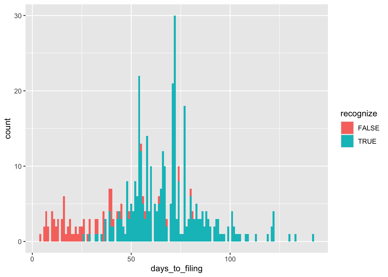
Figure 17.2 depicts the distribution of the number of days between the applicable natural disaster and days to the end of the fiscal period in which it occurs.
michels_2017 |>
  mutate(days_to_period_end = as.integer(next_period_end - eventdate)) |>
  ggplot(aes(x = days_to_period_end, fill = recognize)) +
  geom_histogram(binwidth = 1)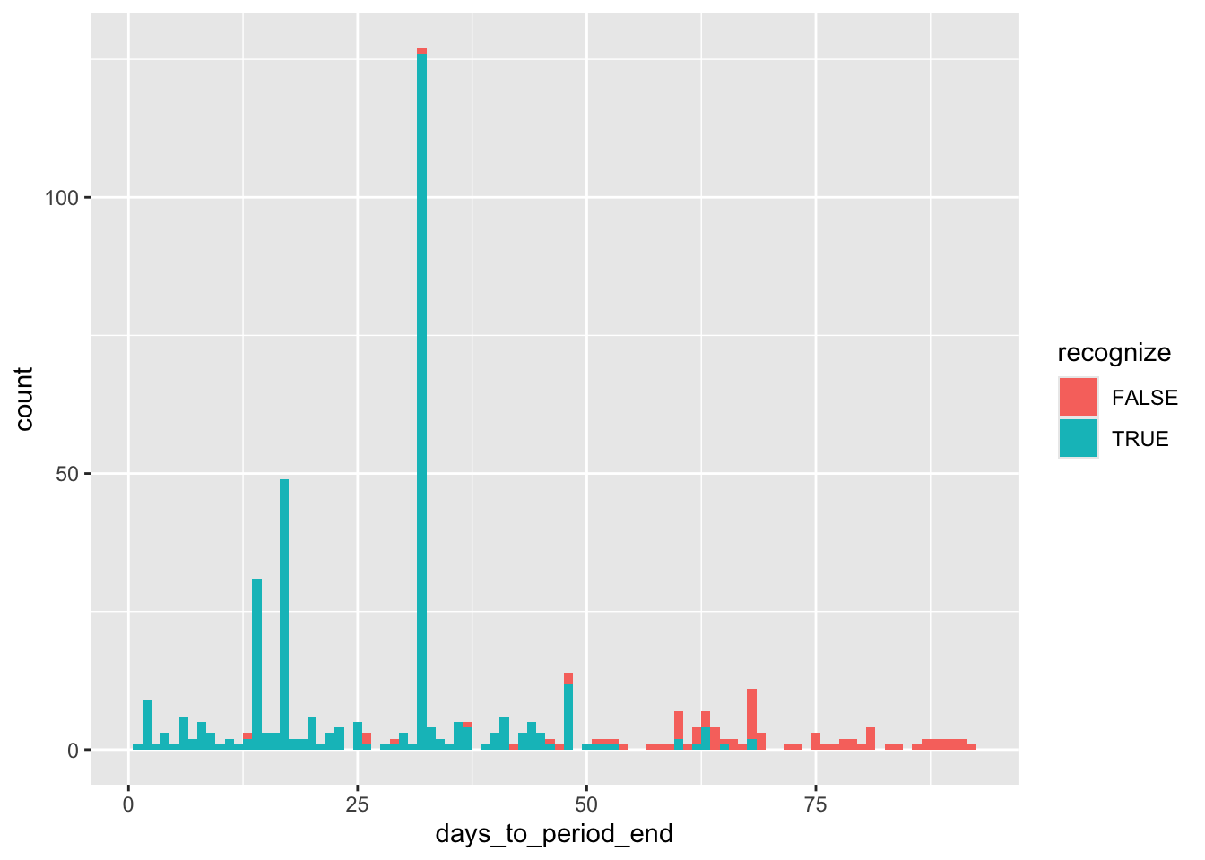
Obviously major natural disasters can affect more than one firm and Table 17.1 provides data on the five most common disaster dates in the Michels (2017) sample.
17.5 Discussion questions
One assumption in Michels (2017) is that whether a natural disaster occurs before or after the balance sheet date of the next filing is random. Do the inherent properties of natural disasters ensure that they are random? Why? If not, how would you evaluate the randomness of natural disasters in the sample of Michels (2017)? Do the analyses above help this evaluation?
Describe what you imagine to be the process from the occurrence of a natural disaster to reporting on that event in the subsequent filing? Do you think this process differs for recognized versus disclosed events?
From the analysis above, it appears that five natural disasters account for 228 observations. A simple Google search for each date and the word “disaster” reveals that these events are Hurricane Katrina (
2005-08-29), Hurricane Ike (2008-09-13), Hurricane Ivan (2004-09-16), Hurricane Charley (2004-08-13), and Hurricane Wilma (2005-10-24). Is it problematic that a small number of disasters accounts for a significant portion of the sample?Where does Michels (2017) get data on natural disasters from? Is there anything that is problematic about this data source? Would it be possible to use another approach to data collection? What challenges would that approach face?
A recurring question in accounting is if it matters whether information is disclosed or recognized. One view is that, if markets are efficient, it should not matter where the information is disclosed, so recognition should not matter relative to disclosure. What assumptions underlie this view? Are there any reasons to believe that they do or do not hold in the setting of Michels (2017)? What are the implications for the ability of Michels (2017) to deliver clean causal inferences? How might materiality criteria differ for disclosed and recognized events? Would differences in these criteria affect the empirical analysis of Michels (2017)?
What causal inferences does Michels (2017) draw? What (if any) issues do you see with regard to these?
Choose a paper that you have seen recently that uses empirical analysis of non-experimental data. (If you cannot choose such a paper, Hopkins et al. (2022) provide one option.) Looking at the abstract of the paper, can you determine whether this paper seeks to draw causal inferences?
Choose what you think the authors regard to be the most important causal inference they draw (or would like to draw) in your chosen paper. Which table or tables provide the relevant empirical analyses? Sketch a rough causal diagram for this causal inference using either discussion in the paper or your own background knowledge to identify important variables. How credible do you find the reported causal inferences to be in light of your causal diagram?
Blinding is difficult to achieve if nature is administering the treatment.↩︎
For more on signalling theory, see Chapter 17 of Kreps (1990).↩︎
If such people exist, then some way of tracking mask-wearing in the control group is perhaps necessary to use an intention-to-treat analysis to estimate the effect of wearing masks.↩︎
Of course, each of these alternatives presents ethical issues that we gloss over, as we are simply trying to illustrate the complexity of specifying treatments.↩︎
The closest equivalent to laboratory studies involving human subjects and medical interventions might be human challenge trials, which present ethical issues and generally involve small sample sizes.↩︎
Indeed, SFAS 123 gave firms the choice to recognize amounts that most firms merely disclosed without reference to any distinctions related to recognition criteria. One possible counterargument to this example is that SFAS 123 was not really about recognition as understood in the conceptual frameworks, but measurement. By measuring the cost of stock-based compensation as zero, there is nothing to recognize. This would seem to be too artful a dodge of the issue and we don’t pursue it further here.↩︎
An illustrative disclosure is found in Microsoft’s 2002 annual report: https://go.unimelb.edu.au/s7d8.↩︎