10 FFJR
This is the published R edition of the book. A Python version of the book is available at era_pl_book.
The (brief!) introduction in Fama et al. (1969) (“FFJR”) confirms that the goal of the paper is to shed light on market efficiency. Prior empirical work had inferred “market efficiency from the observed independence of successive price changes.” In contrast, FFJR focuses on the “speed of adjustment of prices to specific kinds of new information … [specifically] the information (if any) that is implicit in a stock split.” We start this chapter with a brief introduction to the efficient markets hypothesis.
To examine their research question, FFJR conduct one of the earliest event studies. Event studies have a tight connection with notions of efficient markets, especially the “semi-strong” form of the hypothesis offered by Fama (1970), which in turn has important implications for the study of accounting information in capital markets. Thus we use FFJR to provide an initial introduction to event studies, which we revisit in more depth in Chapter 13.
We also use this chapter to introduce the reader to important additional data sets on CRSP, such as those related to dividends and stock splits, and to some R functions for efficiently manipulating data and models (e.g., the unnest() function from the tidyr package). To better understand FFJR, we also provide some background on stock splits and dividends. We then conduct a replication of FFJR and provide exercises for the reader. We conclude the chapter with a guide to this part of the book.
The code in this chapter uses the packages listed below. For instructions on how to set up your computer to use the code found in this book, see Section 1.2. Quarto templates for the exercises below are available on GitHub.
10.1 Efficient capital markets
One of the core ideas in capital market research is the efficient markets hypothesis (EMH). Fama (1991) defines the EMH as “the simple statement that security prices fully reflect all available information.” The EMH is perhaps the most empirically tested proposition in all of social sciences.
In Fama’s formulation, the terms fully reflect and all available information are doing a lot of work. One widely understood implication of the notion that security prices fully reflect a piece of information is that there are no opportunities to generate risk-adjusted profits by trading on that information.1
The EMH is particularly important for accounting research and practice for at least two reasons. First, accounting information is often a component of “all available information” against which the EMH is tested. In particular, Beaver (1998, p. 136) points out that accounting earnings “are widely analyzed by the investment community. No other firm-specific variable receives more attention by the analysts and other capital market participants than earnings.” Second, whether the EMH holds or not has significant implications for preparers, users, and regulators of accounting information.
Richard Thaler identifies two notions of the EMH, which he labels the “price is right” and “no free lunch” principles. The “price is right” principle says asset prices will “fully reflect” available information and thus “provide accurate signals for resource allocation”. The “no free lunch” principle holds that market prices are impossible to predict making it very hard for an investor to beat the market after taking account of risk. The “no free lunch” principle is the variant that is both less demanding of market foresight and more empirically testable.
Most empirical studies of the EMH test the “no free lunch” principle. However, Shiller (1984) laments the existence of “claims that because real returns are nearly unforecastable, the real price of stocks is close to the intrinsic value” and suggest that “this argument for the efficient markets hypothesis represents one of the most remarkable errors in the history of economic thought” (1984, p. 459). In other words, a common fallacy is to conflate the two variants so that evidence for the “no free lunch” variant is adduced as supporting the “price is right” theory.
The “price is right” theory often underlies papers that use event studies to evaluate the merits of corporate policies or regulation. We will discuss some issues with conflation of these two principles in Chapter 13.
10.2 Stock splits
Because much about FFJR and its setting is implicit rather than explicit and might not be clear to a reader entering the field more than fifty years later, we first elucidate some elements of the paper.
Walker (2021, p. 1) describes a stock split as “the issuance of an additional number of shares, at no cost to the shareholder, in proportion to the number of shares already owned. For example, a 2-for-1 split is implemented by a firm issuing one new share for each existing share, thereby doubling the total number of shares outstanding.”
From a fundamental perspective, a stock split might appear to have no economic consequences. Suppose we hold 1,000 shares in a company with an intrinsic value of $500 million and 10 million shares outstanding. Our shares would be worth $50,000 (\(1000 \times 500 \div 10\)). If the company then does a 2-for-1 split so that it now has 20 million shares outstanding, we would have 2,000 shares worth $50,000 (\(2000 \times 500 \div 20\)).
As such, it seems natural to ask why firms engage in stock splits. One explanation posits that, even though there is no underlying effect of a stock splits on the intrinsic value of the firm, markets are not efficient and the stock does not properly adjust for the change in the number of shares, leading to our hypothetical stock holding being worth (say) more than $50,000 after the split. If managers would prefer the firm to have a higher stock market value, this would be a reason to do a stock split.2
But if we assume market efficiency (and being able to calculate the stock-price impact of a stock split is surely a modest level of efficiency), we need to find alternative explanations for stock splits. Walker (2021, p. 2) identifies “two leading explanations”.
The first explanation is the information-signalling hypothesis, which posits that “management uses the split as a channel to signal their private information about the firm’s positive outlook” (Walker, 2021, p. 2). But this is a non-explanation unless there is some underlying effect of a split that is differentially beneficial or costly for firms with private information. For example, a signalling equilibrium might be sustained if a stock split is less costly for firms with better prospects.3 But we need to account for such differences in costs.
The second explanation is the liquidity hypothesis, which “posits that management use a split as a way to improve their stock’s liquidity” (Walker, 2021, p. 2). Delving into the detailed explanations of a liquidity effect of splits would take us too far away from the objectives of this chapter, so we offer a more stylized account that is adequate for our purposes here. We can label this account as a kind of Goldilocks stock price theory whereby a firm’s liquidity is maximized when its stock price trades in a certain range—neither too high nor too low—and that firms tend split their shares if doing so gets their stock prices into this range. For example, if a company’s liquidity is maximized with a stock price around $40, but it is trading at around $80, then a 2-for-1 split would enhance liquidity.
The liquidity hypothesis might fill the gap we identified in the information-signalling hypothesis. If a firm expects to trade at $100 in the future (due to inside information that will come to light later), it might want to do a 2-for-1 split, as a stock at $40 rising to $50 will enjoy better liquidity. But a firm that has inside information and expects to trade closer to $40 in the future (without a split) would be reluctant to do a 2-for-1 split, as it would then expect to trade closer to $20 in the future, and thus would have worse liquidity.
An important element of an event study is the identification of the period during which the market is expected to react to the event information. Like dividends, stock splits will generally be announced prior to their effective date. Fama et al. (1969, p. 7) “define month \(0\) as the month in which the effective date of a split occurs”. Fama et al. (1969, p. 9) mention that for “a random sample of fifty-two splits” from their sample “the median time between the announcement date and the effective date of the split was 44.5 days.” If there is information content in stock splits, we would expect an efficient market to react when the split is announced, not when it is effective. The analyses in FFJR use monthly data, so a median announcement date for splits of 44.5 days before the effective date implies that the median split is announced in month \(-2\). FFJR do not provide details on the distribution of split announcement dates, but some splits may be announced in month \(-1\), while others could occur in month \(-3\) or even earlier.
10.2.1 Discussion question
Consider the following alternative theories.
- Theory A: Firms like to keep their stock price within certain bounds. When the stock price rises above a certain threshold, a firm may initiate a split, announcing it several weeks in advance of its effective date. Firms do not use splits to signal private information about firm prospects.
- Theory B: Firms use splits to signal private information about firm prospects. A firm will announce a split several weeks in advance of its effective date.
- Theory C: Capital market participants don’t fully adjust for the effect of splits, tending to anchor on the pre-split price to some degree. Firms do not use splits to signal private information about firm prospects.
Produce a set of indicative plots (e.g., drawn by hand) for the predicted behaviour of cumulative abnormal returns for assuming that the split is announced in month \(-2\). What impact would variation in the announcement dates relative to the split effective date have on the plots?
10.3 Dividend policy
Black (1976, p. 9) points out that the “Miller-Modigliani theory … says that the dividends a corporation pays do not affect the value of its shares or the returns to investors.” Of course, assumptions underlying the Miller-Modigliani theory include the absence of tax effects or transaction costs. While these assumptions are violated in reality, the violations generally do not provide an explanation for the existence of dividends (e.g., dividends are generally treated unfavourably for tax purposes).
Black (1976, p. 10) summarizes the common understanding of dividends: “For one reason or another, managers and directors do not like to cut the dividend. So they will raise the dividend only if they feel the company’s prospects are good enough to support the higher dividend for some time. And they cut the dividend only if they think the prospects for a quick recovery are poor.” While this theory is “behavioural” (see Thaler, 2015, p. 166, for discussion of this), it has real teeth because managers and directors have inside information and therefore, if they act in accordance with this theory, dividend policy will convey some of this information.
Fama et al. (1969, pp. 2–3) endorse this account of dividends: “Studies … have demonstrated that, once dividends have been increased, large firms show great reluctance to reduce them, except under the most extreme conditions. Directors have appeared to hedge against such dividend cuts by increasing dividends only when they are quite sure of their ability to maintain them in the future, i.e., only when they feel strongly that future earnings will be sufficient to maintain the dividends at their new higher rate. Thus dividend changes may be assumed to convey important information to the market concerning management’s assessment of the firm’s long-run earning and dividend paying potential.”
The connection between stock splits and dividends is not spelt out clearly in FFJR. Fama et al. (1969, p. 2) do say that “in the past a large fraction of stock splits have been followed closely by dividend increases.” Fama et al. (1969, pp. 12–16) offer the following explanation: “When a split is announced or anticipated, the market interprets this (and correctly so) as greatly improving the probability that dividends will soon be substantially increased. (In fact, … in many cases the split and dividend increase will be announced at the same time.)”
Several assumptions are buried in that explanation, which appears to be based on some kind of signalling story.4 For example, why would firms signal future dividend increases using stock splits? And, what are firms signalling with splits when they announce splits and dividend increases at the same time?
10.3.1 Discussion questions
Does the research design of FFJR include the use of a control group? If so, how? What alternative methods could have been used to introduce a control group?
Fama et al. (1969, p. 9) state “the most important empirical results of this study are summarized in Tables 2 and 3 and Figures 2 and 3.” What does Table 3 of FFJR tell us? (Hint: Read p. 11.) Do you find the presentation of Table 3 to be effective?
Consider Table 2 of FFJR. Is it more or less important than Table 3? What is the relationship between Table 2 and Figures 2 and 3?
What statistical tests are used to test the hypotheses of the paper?
10.4 Replication of FFJR
We will now conduct a rough replication of FFJR.5
All the data we will use come from the crsp schema. The new table here is dsedist, which contains information on distributions, including dividends and stock splits.
db <- dbConnect(duckdb::duckdb())

msf <- load_parquet(db, schema = "crsp", table = "msf")
msi <- load_parquet(db, schema = "crsp", table = "msi")
stocknames <- load_parquet(db, schema = "crsp", table = "stocknames")
dsedist <- load_parquet(db, schema = "crsp", table = "dsedist")
Fama et al. (1969, p. 3) “define a ‘stock split’ as an exchange of shares in which at least five shares are distributed for every four formerly outstanding. Thus this definition of splits includes all stock dividends of 25 per cent or greater.”
Fama et al. (1969, p. 3) continue: “Since the data cover only common stocks listed on the New York Stock Exchange, our rules require that to qualify for inclusion in the tests a split security must be listed on the Exchange for at least twelve months before and twelve months after the split. From January, 1927, through December, 1959, 940 splits meeting these criteria occurred on the New York Stock Exchange.” NYSE-listed stocks have exchcd == 1 and ordinary common shares are those for which the first character of shrcd is 1. Data on exchcd and shrcd on various dates is found on crsp.stocknames. The following code creates a table with the permno values and date ranges for the securities meeting these criteria.
nyse_stocks <-
  stocknames |>
  filter(exchcd == 1,
         str_sub(as.character(shrcd), 1L, 1L) == "1") |>
  select(permno, namedt, nameenddt)
We can then use this table to focus splits on these securities.
nyse_splits_raw <-
  splits |>
  inner_join(nyse_stocks,
             join_by(permno, between(exdt, namedt, nameenddt)))
We will need to combine these data with data on returns from crsp.msf. The table crsp.msf contains monthly data indexed by permno and date, where date is the last trading day of the month. The splits in nyse_splits_raw will generally not occur on dates found on crsp.msf, so we need to create a “month” variable so that we can line up observations on crsp.msf and nyse_splits_raw.
To this end we create a table month_indexes that includes the “index” of the month, which will also be used in doing the arithmetic to go backwards and forwards in months. In performing this arithmetic, we use window functions, which are discussed in the documentation for dplyr and in the “Databases” chapter of R for Data Science.6 Here the “index” of a month refers to its placement in the sequence of months found on crsp.msf and crsp.msi.7
month_indexes <-
  msi |>
  mutate(month = as.Date(floor_date(date, 'month'))) |>
  window_order(month) |>
  mutate(month_index = row_number()) |>
  select(date, month, month_index) |>
  collect()
We actually used window functions in Chapter 2 when we used fill() to complete data for calculating market-to-book ratios. It turns out that the window-function functionality made available via the dbplyr package and PostgreSQL (using window_order()) are more powerful in this case than those available via the base dplyr package and tibble data frames (using arrange()), as the dbplyr version allows us to specify a window_frame() over which window functions are applied, as we will see below.
We next bring our splits data (nyse_splits_raw) into R and merge it with month_indexes.
We construct nyse_msf, which is essentially crsp.msf restricted to NYSE stocks and months with non-missing returns, and with the added variable month_index.
nyse_msf <-
  msf |>
  filter(!is.na(ret)) |>
  inner_join(nyse_stocks,
             join_by(permno, between(date, namedt, nameenddt))) |>
  collect() |>
  inner_join(month_indexes, by = "date") |>
  select(permno, month_index, date, ret)
The following code merges data on splits from nyse_splits with data on returns from nyse_msf. We create a variable (month_rel_ex) that measures the number of months between the split and the return.
Because we may have multiple splits for a given permno in nyse_splits (each with a different exdt) and each will be joined with multiple return months in nyse_msf, we will have a many-to-many relationship between rows in nyse_splits and rows in nyse_msf. To suppress a warning that dplyr issues in such cases, we indicate that we anticipate such matches by specifying relationship = "many-to-many" as an argument to left_join().
However, we want to ensure that we have just one row for each (permno, exdt, month_rel_ex) combination:
# A tibble: 1 × 2
  n_rows      n
   <int>  <int>
1      1 641836
Fama et al. (1969, p. 3) “decided, arbitrarily, that in order to get reliable estimates of the parameters that will be used in the analysis, it is necessary to have at least twenty-four successive months of price-dividend data around the split date.” Note that Fama et al. (1969) actually look at 12 months before and 12 months after the split, so including the month of the split, we have 25 months. The table split_sample imposes this restriction and, by doing a semi_join() of this with split_return_data, we create split_returns, which contains the data from crsp.msf for our sample of splits.
The sample of Fama et al. (1969, p. 4) comprises 940 splits for 622 securities. The output from the code below suggests that our sample is slightly larger, perhaps due to changes in the underlying data since 1966.
[1] 626[1] 948We follow the basic approach of FFJR in estimating excess returns. FFJR estimate a market model by regressing the log of gross returns of each stock on the log of gross returns of a market index and taking the residual.
The market index used in Fama et al. (1969, p. 4) is Fisher’s Combination Investment Performance Index, which is made available as Table A1 in Fisher (1966). To use this table, which is not available in a machine-readable form, we would have to type in the hundreds of numbers contained therein. Instead of doing that, we will use one of the standard indexes provided by CRSP in crsp.msi. There are two widely used indexes on crsp.msi: vwretd provides the value-weighted return including distributions and ewretd provides the equal-weighted return including distributions. A value-weighted index weights each security in the portfolio based on its market value at the time of portfolio formation, while an equal-weighted index puts equal weight on each security in the portfolio regardless of its market value. For our base analysis, we will focus on vwretd.
Fama et al. (1969, pp. 4–5) express concern about non-zero excess returns causing “specification error” and exclude “fifteen months before the split for all securities and fifteen months after the split for splits followed by dividend decreases.” We partially implement this by excluding fifteen months before the split for all securities, but not excluding any months after the split, as this requires data on dividends that would not have been available at the time of the split—which we do not compile until later (see below)—and thus induces additional look-ahead issues.
Note that because a (permno, date) combination may appear for more than one split, and be within fifteen months before the split for one split, and not so for another split, we need to aggregate data across such observations. The following code sets exclude to true if the (permno, date) combination is within fifteen months before any split for that stock.
The following code adds exclude to the data from split_returns. Note that we need to select distinct values for return data from split_returns, as a (permno, date) combination may appear more than once, but with different values of month_rel_ex due to it relating to more than one split. Note also that we do not simply drop rows from the data set where exclude is TRUE, as we want to calculate abnormal returns for these months. Instead, we merely exclude these observations from the regression analysis by specifying subset = !exclude.
split_returns_reg <-
  split_returns |>
  inner_join(omit_returns, by = c("permno", "date")) |>
  select(permno, date, ret, exclude) |>
  distinct()
The next step is to estimate regressions by permno. Like FFJR, we estimate a market model by regressing the log of gross returns of each stock on the log of gross returns of a market index. In the code below, we make extensive use of ideas from the “many models” chapter of the first edition of R for Data Science and you may find it helpful to read that chapter.8
Because we want to fit one model for each permno, we facilitate this by using nest() to put all the data for each value of permno (other than the value of permno) into a single column. We can then use map() from the purrr library to create a new column fit that contains a fitted linear (OLS) model for each permno value. If we apply predict() to the model, we will get fitted values only for those observations used to estimate the model, which will mean we will not have predicted values for months within fifteen months before the split. Instead, we need to supply data for all observations as the second argument (newdata) of the predict function. To do this, we use map2() from the purrr library and store the result in the variable predicted.
Note that predicted will be a list-column in which each element is a vector of predicted values using the market model for the applicable permno. We can use unnest() from the tidyr package to “expand” the data frame so that each row relates to a given (permno, date) pair. Finally, we calculate excess returns by subtracting predicted from the actual value of lpr and store the result in the column named resid.
abnormal_returns <-
  split_returns_reg |>
  left_join(index_returns, by = "date") |>
  mutate(lpr = log(1 + ret),
         lm = log(1 + vwretd)) |>
  select(permno, date, lpr, lm, exclude) |>
  nest(data = !permno) |>
  mutate(fit = map(data, \(x) lm(lpr ~ lm, data = x, subset = !exclude,
                              na.action = "na.exclude"))) |>
  mutate(predicted = map2(fit, data, \(x, y) predict(x, newdata = y))) |>
  unnest(cols = c(predicted, data)) |>
  mutate(resid = lpr - predicted) |>
  select(permno, date, resid)
To facilitate joining abnormal_returns with nyse_splits, we create a version of nyse_splits with start and end columns that indicate the month_index of the first and last months that we want abnormal returns for (i.e., within 30 months of the split).
nyse_splits_join <-
  nyse_splits |>
  mutate(start = ex_month_index - 30,
         end = ex_month_index + 30)
We can combine abnormal_returns with nyse_splits, but before doing so, we need to pull in month_index for each date from month_indexes. We join abnormal_returns with nyse_splits using permno and month_index between start and end.
table2_data <-
  abnormal_returns |>
  inner_join(month_indexes, by = "date") |>
  inner_join(nyse_splits_join,
             join_by(permno, between(month_index, start, end))) |>
  mutate(month_gap = month_index - ex_month_index) |>
  select(permno, exdt, month_gap, resid)
Before proceeding, we check that we have just one row for each split (permno and exdt) and relative month (month_gap).9
# A tibble: 1 × 2
n_rows n
<int> <int>
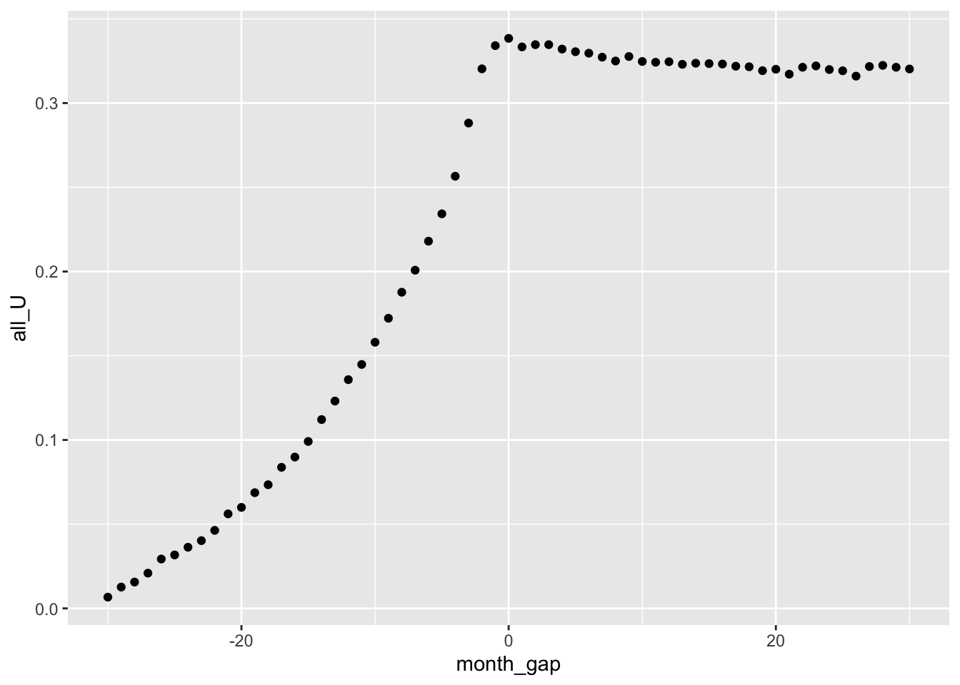
1 1 57986We now have the data we need to produce Figure 10.1, our analogue of Figure 2b from Fama et al. (1969, p. 13).
10.4.1 Data on dividends
Most columns of Table 2 of FFJR and all plots in Figure 3 of FFJR require data on dividends. We collect data on dividends from dsedist.10 Ordinary dividends are distinguished from other distributions (e.g., liquidating dividends or exchanges and reorganizations) by the first digit of distcd, which is 1 for ordinary dividends.
It turns out that there can be more than one dividend paid in a given month for a given security, so we aggregate dividends by (permno, month).
For each month, FFJR define “the dividend change ratio as total dividends (per equivalent unsplit share) paid in the twelve months after the split, divided by total dividends paid during the twelve months before the split” Fama et al. (1969, p. 8). So, for each month \(t\), we want to sum up dividends from month \(t -11\) to month \(t\) and also dividends for months \(t + 1\) through \(t + 12\).
Care is needed to calculate dividends “per equivalent unsplit share” as a firm paying 80 cents per share each quarter prior to a 2-for-1 split should be considered to have increased its dividends if it paid 45 cents per share (i.e., 90 cents per original share) in each quarter after the split. The variable cfacshr from msf allows us to make the necessary adjustment.11
If no dividends are paid on a stock in a given month, we set divamt to zero; this allows us to distinguish months where a stock is not an NYSE stock on crsp.msf (missing from this table) from ones where it is, but pays no dividend that month (i.e., zero divamt).12
nyse_divs_raw <-
  msf |>
  inner_join(nyse_stocks, by = "permno") |>
  filter(between(date, namedt, nameenddt)) |>
  mutate(month = as.Date(floor_date(date, 'month'))) |>
  select(permno, date, month, cfacshr) |>
  left_join(div_months, by = c("permno", "month")) |>
  mutate(divamt = coalesce(divamt / cfacshr, 0)) |>
  select(permno, month, divamt)
The following code aggregates the variables needed to calculate the dividend change ratio mentioned above: dividends paid in the twelve months after the split and dividends paid during the twelve months before the split.
In this case, we specify group_by(permno) as we want windows to be applied on a by-PERMNO basis (i.e., when calculating trailing and forward dividends, we are only interested in dividends related to a single PERMNO) and then window_order(month), as we want to arrange the data within each window by month so that “go back 11 months” is meaningfully defined. In the next step, we specify window_frame(from = -11, to = 0) to indicate that in the subsequent calculation, we want to include values from \(t - 11\) to \(t\) in the window.13 This drives the values considered in the subsequent mutate() step, which calculates div_trailing and mths_trailing. Note that na.rm = TRUE is always the case for SQL (which this code is ultimately translated into) and that n() counts the numbers of rows included in the window.
We then respecify the window using window_frame(from = 1, to = 12) so that we can calculate div_forward and mths_forward.
Finally, to exclude cases where, say, a stock has listed within the last twelve months or delists in the subsequent twelve months and thereby perhaps makes the calculation of the dividend change ratio less meaningful, we use filter(mths_trailing == 12, mths_forward == 12). Finally, we ungroup to remove the group_by(permno) grouping that we no longer need, select the variables of interest, and then collect the data.
nyse_divs <-
  nyse_divs_raw |>
  group_by(permno) |>
  window_order(month) |>
  window_frame(from = -11, to = 0) |>
  mutate(div_trailing = sum(divamt, na.rm = TRUE),
         mths_trailing = n()) |>
  window_frame(from = 1, to = 12) |>
  mutate(div_forward = sum(divamt, na.rm = TRUE),
         mths_forward = n()) |>
  filter(mths_trailing == 12, mths_forward == 12) |>
  ungroup() |>
  select(permno, month, div_trailing, div_forward) |>
  collect()
Now that we have data on div_trailing and div_forward for every (permno, month) combination on NYSE, we can use these data to calculate the dividend change ratio (div_ratio) for each of the split months on nyse_splits.
Fama et al. (1969, p. 8) measure dividend changes “relative to the average dividends paid by all securities on the New York Stock Exchange during the relevant time periods. … Dividend ‘increases’ are then defined as cases where the dividend change ratio of the split stock is greater than the ratio for the Exchange as a whole.” We calculate the “market” dividend change ratio (mkt_div_ratio) by averaging the div_trailing and div_forward values for each month across all stocks.
We can then combine data on split- and market-level dividend change ratios for each month in which there is a split to calculate up_div, which is an indicator for the dividend change ratios for a stock undergoing a split being greater than that for the market in that month.
Fama et al. (1969, p. 9) do not pretend that their measure of dividend increases is perfect and merely use it as “a simple and convenient way of … classifying year-to-year dividend changes for individual securities.”14
dividends_file <-
  split_firm_dividends |>
  inner_join(div_mkt, by = "month") |>
  select(permno, exdt, div_ratio, mkt_div_ratio) |>
  mutate(up_div = div_ratio >= mkt_div_ratio)
Finally, we can combine data on relative dividend change ratios with abnormal return data.
We can now produce Figure 10.2, our analogue of Figure 3c from Fama et al. (1969, p. 15).
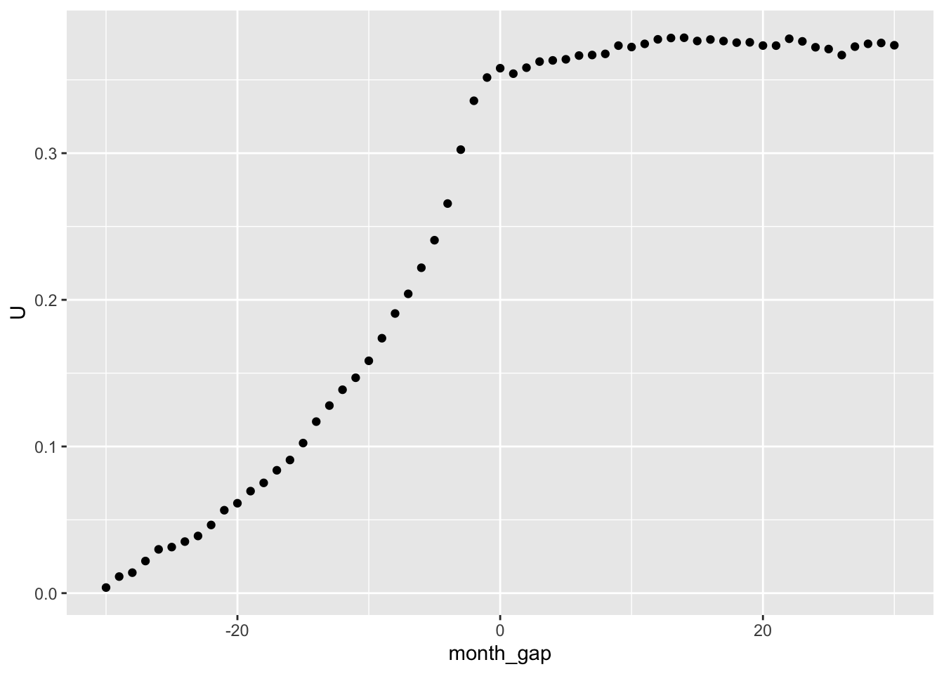
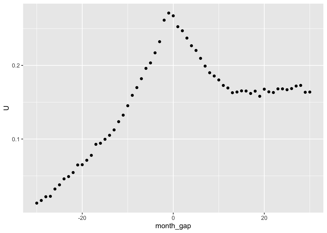
Figure 10.3 provides our equivalent of Figure 3d from Fama et al. (1969, p. 15).
10.4.2 Discussion questions and exercises
“In the past a large fraction of stock splits have been followed closely by dividend increases—and increases greater than those experienced at the same time by other securities in the market.” What evidence to support this claim (if any) is provided by FFJR? Do we see evidence consistent with this in the data underlying our replication above?
-
Consider the three alternative theories below. Suggest tests that could distinguish which of these theories best explains observed phenomena. Which theory best aligns the theory proposed by FFJR? How would this theory need to be modified to comport better with the theory proposed by FFJR?
- Theory \(A'\): Firms like to keep their stock price within certain bounds. When the stock price rises above a certain threshold, a firm may initiate a split, announcing it several weeks in advance of its effective date. Firms do not use splits to signal private information about firm prospects. Pre-split stock prices may be driven by information that suggests an imminent increase in dividends.
- Theory \(B'\): Firms use splits to signal private information about firm prospects. A firm will announce a split several weeks in advance of its effective date. Firms may also use dividend changes to signal private information about firm prospects.
- Theory \(B^{''}\): Firms use splits to signal private information about future dividend increases, which in turn signal private information about firm prospects. A firm will announce a split several weeks in advance of its effective date.
On p. 17 of Fama et al. (1969), it is argued that “our data suggest that once the information effects of associated dividends are properly considered, a split per se has no net effect on common stock returns.” Is it clear what meaning the words “per se” have in this sentence? Does FFJR provide persuasive evidence in support of this claim? Describe how you might test this claim using the richer data available today. What data would you use beyond that used in FFJR?
How do the figures produced above compare with their equivalents in FFJR? What might account for any differences?
In the analysis above we used
vwretdas the market index. Modify the code above to instead useewretd. Do you observe any changes in the resulting figures? Which do you believe is the better market index for these plots? Why?
10.5 Capital markets research in accounting
This part of the book focuses on capital markets research, which is arguably the area in which academic research has most contributed to our understanding of real-world accounting phenomena. One goal of this part is to provide a solid introduction to classical ideas and papers related to capital markets research in accounting.
This chapter introduced the idea of efficient capital markets and focuses on Fama et al. (1969), one of the earliest event studies in capital markets research. The next two chapters—Chapters 11 and 12—cover two seminal papers, Ball and Brown (1968) and Beaver (1968), respectively. While the first three chapters of this part study papers from more than 50 years ago, we believe that they provide an excellent introduction to the foundations of research design that remain relevant to this day.
Chapter 13 builds on the three previous chapters in providing more depth on event studies, including coverage of how event studies have evolved since Fama et al. (1969). Chapter 14 examines post-earnings announcement drift, a much-studied anomaly in the pricing of accounting information in capital markets. Chapter 15 goes deeper into the measurement of accruals, a critical element of financial accounting, and also provides an opportunity to explore simulation analysis in more detail. Chapter 16 explores earnings management, which has been the focus of significant body of accounting research over several decades, and also provides an opportunity to understand issues related to measurement in research and the power of statistical tests.
Another deeper implication of the EMH is that prices should be “correct” in some sense.↩︎
In some cases, managers might benefit from a lower post-split stock market value, say, if they want to purchase shares themselves after the split.↩︎
For more on signalling theory, see Chapter 17 of Kreps (1990).↩︎
Evidence that FFJR have a signalling story in mind comes from subsequent sentences in the paper.↩︎
We thank James Kavourakis for an earlier replication effort that helped us in preparing this code.↩︎
Also see https://www.postgresql.org/docs/current/tutorial-window.html.↩︎
Note that we are operating on remote data here, so we use
window_order()instead ofarrange()when using window functions. In fact,window_order()offers power that is not available with local data frames. In Chapters 6 and 8, we useddbplyrimplicitly when connecting to databases through thedplyrpackage, butwindow_order()is not “re-exported” by thedplyrpackage and thus we needed to invokelibrary(dbplyr)above.↩︎There is no close equivalent in the second edition of R for Data Science. Instead readers of that book are directed to Tidy Modeling with R https://www.tmwr.org (Kuhn and Silge, 2022).↩︎
It seems that by using an inequality join (i.e.,
join_by(between())), a “many-to-many” check is not applied automatically.↩︎The table
crsp.dsedistis a subset of the tablecrsp.dsefocused on distributions.↩︎Note that, as
cfacshrcomes fromcrsp.msf, it is presumably the value applicable at the end of the month. It seems possible that a firm could pay a dividend and then split its stock in the same month, in which case applying the end-of-monthcfacshrto the dividend would be incorrect. For the purposes of this chapter, we ignore this issue, but a careful researcher would investigate further when conducting a proper research study.↩︎We want to do this for every month that a security was an NYSE security, so we start from
msfand join withnyse_stocks. Note that we cannot use thenyse_msfdata frame created above because this is a local data frame and we are using remote data fromdiv_monthsin this analysis. This may be a case where a little duplicate code is preferred to shifting data from a local machine to a remote one or vice versa.↩︎Like
window_order(),window_frame()is only available for remote data frames because it relies on the SQL backend to provide functionality not available with local data frames.↩︎See Fama et al. (1969, p. 9) for discussion of some limitations of the measure.↩︎