12  Beaver (1968)

In this chapter, we cover Beaver (1968), the second winner of the Seminal Contributions to Accounting Literature Award. Beaver (1968) followed Ball and Brown (1968) and examines whether investors appear to react to earnings announcements.

Beaver (1968) uses two approaches to measure investor reaction. The first approach measures market reaction using trading volume and the second uses the squared return residuals, where return residuals are the difference between observed returns and fitted returns using a market model (1968, p. 78).

In this chapter, we start with a close study of Beaver (1968) itself before introducing Bamber et al. (2000), wich provides a critique of Beaver (1968). We then conduct a “replication” of Beaver (1968) using a more recent sample period and use that replication to think about Beaver (1968) and the issues raised by Bamber et al. (2000).

Tip

The code in this chapter uses the packages listed below. For instructions on how to set up your computer to use the code found in this book, see Section 1.2. Quarto templates for the exercises below are available at https://github.com/iangow/far_templates.

library(dplyr)
library(DBI)
library(ggplot2)
library(farr)
library(lubridate)  # For year()
library(tidyr)      # For fill()
library(dbplyr)     # For copy_inline()

12.1 Market reactions to earnings announcements

Results for the volume analysis are provided in Figures 1 and 3 of Beaver (1968). Figure 1 provides analysis of unadjusted volume and Figure 3 provides analysis of residual volume, which is calculated as the residual from a kind of “volume market model” (see p. 76 of Beaver, 1968). Figure 6 contains the results of the analysis of return residuals.

Some aspects of the Beaver (1968) are confusing unless read closely, so we provide some explanation here. The sample in Beaver (1968) comprises 506 earnings announcements for 143 firms. Each earnings announcement is associated with a 17-week announcement window (\(t = -8, \dots, +8\)), which Beaver (1968) calls the “report period”. Observations on returns and volumes within the sample period for a given firm, but outside report periods for that firm, make up the non-report period for that firm. There are 261 periods in the sample as there are 261 weeks between the start of 1961 and the end of 1965.

Figure 2 of Beaver (1968) provides information about the distribution of residual volume measured for each of the 261 weeks. The formula in the top-left of this figure is not strictly correct, as the number of firms for which residual volume would be available would generally be less than 143 due to the exclusion of values for firms during their report periods.

Figures 4 and 7 of Beaver (1968) are used to support inferences discussed in the text of the paper. The dashed line in Figure 4 is presumably around the value of 179 (\(179 \approx 506 \times 0.354\), as \(35.4\%\) of residual volume values in the non-report period are positive [see discussion on p. 76]), even though the mean of residual volume is (by definition) equal to zero during the non-report period. The dashed line in Figure 7 is presumably around the value of 132 (\(132 \approx 506 \times 0.26\), as \(26\%\) of return residuals in the non-report period exceed one [see footnote 26 on p. 80]), even though the mean value is (by definition) equal to one during the non-report period. Note that the figures in Beaver (1968) would have been created using tools such as rulers, pens, and scissors rather than anything like ggplot2.

12.1.1 Discussion questions

1. How do the research questions of Beaver (1968) and Ball and Brown (1968) differ? If there is overlap, do you think that one paper provides superior evidence to the other? Or are they just different?

2. What differences are there in the data (e.g., sample period) used in Beaver (1968) from the data used in Ball and Brown (1968)? Why do these differences exist?

3. Do the reasons given by Beaver (1968) for his sample selection criteria seem reasonable? Do you think these were made prior to looking at results? (Why or why not?) Does it matter at what stage in the research process these decisions were made?

4. Which do you think is the better variable—price or volume—for addressing the research questions of Beaver (1968)? Do you think it is helpful to have both variables?

5. Beaver (1968) compares event-week volume and volatility with their average equivalents in non-event periods. Ball and Shivakumar (2008) “quantify the relative importance of earnings announcements in providing new information to the share market” and argue that earnings announcements provide relatively little of this information. If volume is a measure of information content, what does Figure 1 of Beaver (1968) imply regarding the proportion of information conveyed during earnings announcement weeks? Can this be reconciled with reported results in Beaver (1968) and the arguments in Ball and Shivakumar (2008)?

6. Beaver (1968) discusses the statistical significance of his results on p. 77 (residual volume analysis) and pp. 81-82 (return residual analysis). Why do think Beaver (1968) uses the approaches discussed there? How might you evaluate statistical significance more formally if you were writing the paper today?

7. The primary analyses in Beaver (1968) are provided in plots. While the cost of producing plots has surely plummeted since 1968, we generally do not see primary analyses presented as plots today. Why do you think this is the case?

12.2 A re-evaluation of Beaver (1968)

Bamber et al. (2000) analyse the setting of Beaver (1968) using the same sample—announcement of annual earnings between 1961 and 1965—but consider modifications to sample selection and empirical tests. Bamber et al. (2000) replicate the results of Beaver (1968), but argue that these are not robust to two alternative research design choices. First, they find that Beaver’s “focus on mean effects obscures the fact that most individual earnings announcements are not associated with unusual price reactions” (2000, p. 105). Second, rather than apply Beaver’s sample selection criteria, Bamber et al. (2000, p. 105) “choose an alternative set of firms that would have been at least equally interesting at the time when there was no empirical evidence on the information content of any firms’ [sic] earnings announcements—the era’s Fortune 200 firms.”

Bamber et al. (2000) suggest that “had the initial information content studies made different research design choices … the apparent information content would have been much less dramatic, and perhaps even non-existent. [After early studies] the conclusion that earnings announcements convey new information to the market soon became the received wisdom.”

In this chapter, we will revisit the question of whether “earnings announcements convey new information to the market” using the basic research design of Beaver (1968) and the same focus on NYSE firms, but using all of them (subject to data availability), focusing on recent earnings announcements—specifically those related to fiscal periods ending between 1 January 2010 and 31 December 2019—and making a few simplifications to the empirical analysis of Beaver (1968).

12.2.1 Core set of events from Compustat

We begin by connecting to the several tables we will use in our analysis.

PostgreSQL

db <- dbConnect(RPostgres::Postgres(), bigint = "integer")

dsf <- tbl(db, Id(schema = "crsp", table = "dsf"))
dsi <- tbl(db, Id(schema = "crsp", table = "dsi"))
msf <- tbl(db, Id(schema = "crsp", table = "msf"))
msi <- tbl(db, Id(schema = "crsp", table = "msi"))
ccmxpf_lnkhist <- tbl(db, Id(schema = "crsp", table = "ccmxpf_lnkhist"))
stocknames <- tbl(db, Id(schema = "crsp", table = "stocknames"))

funda <- tbl(db, Id(schema = "comp", table = "funda"))
fundq <- tbl(db, Id(schema = "comp", table = "fundq"))

parquet

db <- dbConnect(duckdb::duckdb())

dsf <- load_parquet(db, schema = "crsp", table = "dsf")
dsi <- load_parquet(db, schema = "crsp", table = "dsi")
msf <- load_parquet(db, schema = "crsp", table = "msf")
msi <- load_parquet(db, schema = "crsp", table = "msi")
ccmxpf_lnkhist <- load_parquet(db, schema = "crsp", table = "ccmxpf_lnkhist")
stocknames <- load_parquet(db, schema = "crsp", table = "stocknames")

funda <- load_parquet(db, schema = "comp", table = "funda")
fundq <- load_parquet(db, schema = "comp", table = "fundq")

Our next task is to collect the set of earnings announcements that we will use in our analysis. Beaver (1968) obtained earnings announcement dates from the Wall Street Journal Index (1968, p. 72), but for our newer sample period we can use the field rdq found on the Compustat quarterly data file (comp.fundq). Following Beaver (1968), we focus on annual earnings announcements.¹

first_date <- "2010-01-01"
last_date <- "2019-12-31"

earn_annc_dates <-
  fundq |>
  filter(indfmt == "INDL", datafmt == "STD",
         consol == "C", popsrc == "D") |>
  filter(!is.na(rdq), fqtr == 4L) |>
  select(gvkey, datadate, rdq) |>
  filter(between(datadate, first_date, last_date)) |>
  collect()

The data frame earn_annc_dates provides our set of event dates. Like Beaver (1968), we also need a set of non-event dates for comparison. Implicitly, Beaver (1968) used weeks \((-8, \dots, -1)\) and \((+1, \dots, +8)\) as non-event weeks. In our mini-study, we will use daily data and look at dates between 20 trading days before and 20 trading days after the announcement of earnings.

For our purposes, a trading day (or trading date) will be a date on which CRSP stocks traded. In other words, dates found on crsp.dsf will be considered trading days. In the last chapter, we confirmed that the same dates are found on crsp.dsf and crsp.dsi, so we can use either. Because each date is only found once on crsp.dsi, we will use that smaller table.

12.2.2 Replication for a single event

For concreteness, we begin with a focus a single earnings announcement: CTI BioPharma Corporation, a biopharmaceutical company with GVKEY of 064515 that announced earnings for the year ending 31 December 2017 on 2018-03-04.

single_event <-
  earn_annc_dates |>
  filter(gvkey == "064515", rdq == "2018-03-04")

First, we need to map our GVKEY to a PERMNO and we use ccm_link as seen in Chapter 7 for this purpose:

ccm_link <-
  ccmxpf_lnkhist |>
  filter(linktype %in% c("LC", "LU", "LS"),
         linkprim %in% c("C", "P")) |>
  rename(permno = lpermno) |>
  mutate(linkenddt = coalesce(linkenddt, max(linkenddt, na.rm = TRUE))) |>
  collect()

Now we can make our link table, which here covers just one firm.

single_event_link <-
  single_event |>
  inner_join(ccm_link, join_by(gvkey, rdq >= linkdt, rdq <= linkenddt)) |>
  select(gvkey, datadate, permno) 

Next, we need to identify the dates for which we need return and volume data, namely the period extending from twenty trading days before the earnings announcement to twenty days after.

One issue we might consider is: when (at what time) did the firm announce earnings? If the firm announced after trading hours, then the first opportunity that the market would have to react to that information will be the next day. But, for our purposes, we don’t need to be this precise and we will assume that, if a firm announces earnings on a trading date, then that date will be trading day zero.

A second issue to consider is: What do we do with announcements that occur on non-trading dates? For example, CTI BioPharma Corporation’s earnings announcement occurred on Sunday (a firm might also announce earnings on a public holiday). In this case, it seems reasonable to assume that trading day zero will be the next available trading day (e.g., if a firm announces earnings on Sunday and the Monday is a trading date, then that Monday would be the relevant day zero).

The final issue relates to the arithmetic of counting forward and backwards. Suppose a firm announced earnings on 2018-03-05, a Monday. Because that date is a trading date, day zero would be 2018-03-05. But day \(-1\) would be 2018-03-02, as 2018-03-03 and 2018-03-04 are non-trading dates (a Saturday and a Sunday, respectively).

Let’s address the last issue first. If we take the dates on crsp.dsi, and order the data by date, then we can create a variable td using the row_number() function where td stands for “trading day” and represents, for each date, the number of trading days since the start of crsp.dsi.

trading_dates <-
  dsi |>
  select(date) |>
  collect() |>
  arrange(date) |>
  mutate(td = row_number())

In our example, 2018-03-05 has td equal to 24333 and subtracting 1 from that td gives 24332, which is associated with 2018-03-02.

trading_dates |>
  filter(date >= "2018-02-27") 

# A tibble: 1,471 × 2
   date          td
   <date>     <int>
 1 2018-02-27 24329
 2 2018-02-28 24330
 3 2018-03-01 24331
 4 2018-03-02 24332
 5 2018-03-05 24333
 6 2018-03-06 24334
 7 2018-03-07 24335
 8 2018-03-08 24336
 9 2018-03-09 24337
10 2018-03-12 24338
# ℹ 1,461 more rows

Similar calculations can be done with any number of trading days.² This solves the final issue, but what about the second issue of announcements on non-trading dates? To address this, we make a table annc_dates as follows:

1. Create a table with all possible announcement dates. (In this case, we use the seq function to create a list of all dates over the period represented on crsp.dsi.)
2. Where possible, line these dates up with dates (and their associated td values) on trading_dates. (The “where possible” translates into using a left_join() in this case.)
3. Fill in the missing td entries by grabbing the next available td. (For this, we use the fill() function from the tidyr package.)

min_date <- 
  trading_dates |>
  summarize(min(date, na.rm = TRUE)) |>
  pull()

max_date <- 
  trading_dates |>
  summarize(max(date, na.rm = TRUE)) |>
  pull()

annc_dates <-
  tibble(annc_date = seq(min_date, max_date, 1)) |>
  left_join(trading_dates, by = join_by(annc_date == date)) |>
  fill(td, .direction = "up")

To illustrate how we can use this table, let’s return to our earnings announcement on 2018-03-04 where we’re interested in returns running over the window from \(t-20\) to \(t+20\). We can see below that 2018-03-04 has td equal to 24333 (this because the relevant day zero is 2018-03-05, which has td of 24333). So we identify \(t-20\) as the date with td equal to 24313 and \(t+20\) as the date with td equal to 24353.

trading_dates |>
  filter(td %in% c(24313, 24353))

# A tibble: 2 × 2
  date          td
  <date>     <int>
1 2018-02-02 24313
2 2018-04-03 24353

days_before <- 20L
days_after <- 20L
  
single_event_window <-
  single_event |>
  left_join(annc_dates, by = join_by(rdq == annc_date)) |>
  mutate(start_td = td - days_before, 
         end_td = td + days_after) |>
  inner_join(trading_dates, by = join_by(start_td == td)) |>
  rename(start_date = date) |>
  inner_join(trading_dates, by = join_by(end_td == td)) |>
  rename(end_date = date,
         event_td = td) |>
  select(-start_td, -end_td)

single_event_window 

# A tibble: 1 × 6
  gvkey  datadate   rdq        event_td start_date end_date  
  <chr>  <date>     <date>        <int> <date>     <date>    
1 064515 2017-12-31 2018-03-04    24333 2018-02-02 2018-04-03

We then merge this data set with our link table to create a table that we can link with CRSP.

single_event_window_permno <-
  single_event_window |>
  inner_join(single_event_link, by = c("gvkey", "datadate"))

Now that we have the dates and PERMNO for which we want CRSP data, we now need to go grab those data. Here, we are interested in stock and market returns (ret and ret_mkt, respectively) and volume (vol) for each date.

mkt_rets <-
  dsf |>
  inner_join(dsi, by = "date") |>
  mutate(ret_mkt = ret - vwretd) |>
  select(permno, date, ret, ret_mkt, vol)

We next merge mkt_rets with our event data to create single_event_crsp. Note that we have a slight problem here because we want to merge data on events, which is found in the local data frame single_event_window_permno, with data from crsp.dsf, which is found in the WRDS database, which we have as a remote data frame. One approach would run collect() on crsp.dsf to turn it into a local data frame, but this would be very cumbersome (it’s about 20GB in size). Another approach would be to copy the local data frame to the WRDS PostgreSQL server, but WRDS does not allow us to write data to the server. Fortunately, we can use the copy_inline() function from the dbplyr package, which allows us to create something similar to a temporary table on the server using local data.³

PostgreSQL

single_event_crsp <-
  copy_inline(db, single_event_window_permno) |>
  inner_join(mkt_rets, by = "permno") |>
  filter(date >= start_date, date <= end_date) |>
  select(gvkey, datadate, event_td, date, ret, ret_mkt, vol)

parquet

single_event_crsp <-
  copy_to(db, single_event_window_permno) |>
  inner_join(mkt_rets, by = "permno") |>
  filter(date >= start_date, date <= end_date) |>
  select(gvkey, datadate, event_td, date, ret, ret_mkt, vol)

The final step is to convert certain date variables into event time. For example, 2018-02-02 has td of 21313, but this isn’t particularly meaningful here. What is important is that 2018-02-02 represents \(t-20\) for the earnings announcement on 2018-03-04. To convert each date to a “relative trading day”, we just need to join our single_event_crsp table with trading_dates to get the relevant td data, then subtract the event_td from the retrieved td. The follow code does this and puts the results in a new data frame.

single_event_tds <-
  single_event_crsp |>
  collect() |>
  inner_join(trading_dates, by = "date") |>
  mutate(relative_td = td - event_td) |>
  select(-event_td, -td) 

Now we can do a simple plot (Figure 12.1) of the trading volume (vol) against the number of trading days from the earnings announcement (relative_td).

single_event_tds |>
  ggplot(aes(x = relative_td, y = vol)) + 
  geom_line()

Figure 12.1: Return volatility around earnings announcement: Single event

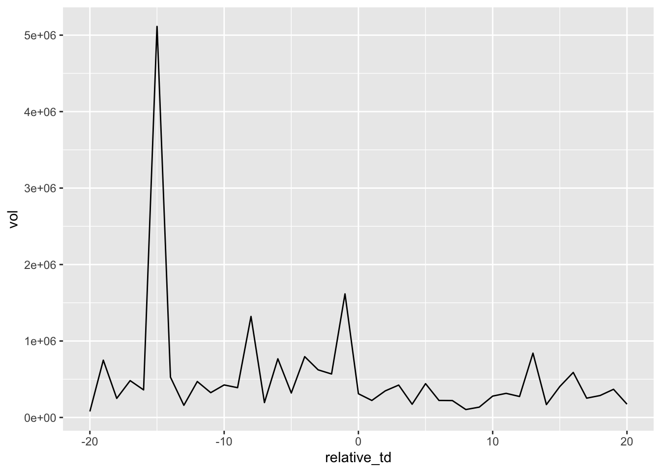
Interestingly there is no volume spike on the earnings announcement date, but there is a small spike just before it and a larger one in February, when CTI BioPharma executed a stock offering. Note that there was actually no Sunday earnings announcement in this case; CTI BioPharma actually announced earnings at 4:01 pm EST on 7 March 2018 suggesting that the rdq on Compustat is simply incorrect.

12.2.3 Replication for the full sample

We now retrace the steps we took above, but using the full data set earn_annc_dates in place of the single_event data frame. While our goal is not to replicate Beaver (1968) precisely, we follow Beaver (1968) in focusing on NYSE-listed firms. Data on the exchanges that firms are listed on is found in exchcd, which is found on crsp.stocknames.⁴

nyse <-
  stocknames |> 
  filter(exchcd == 1) |>
  select(permno, namedt, nameenddt) |>
  collect()

We add PERMNOs from ccm_link and limit the data to NYSE firms.

earn_annc_links <-
  earn_annc_dates |>
  inner_join(ccm_link, join_by(gvkey, rdq >= linkdt, rdq <= linkenddt)) |>
  semi_join(nyse, join_by(permno, rdq >= namedt, rdq <= nameenddt)) |>
  select(gvkey, datadate, rdq, permno)

We add the relevant dates using annc_dates and trading_dates.

earn_annc_windows <-
  earn_annc_dates |>
  inner_join(annc_dates, by = join_by(rdq == annc_date)) |>
  mutate(start_td = td - days_before, 
         end_td = td + days_after) |>
  inner_join(trading_dates, by = join_by(start_td == td)) |>
  rename(start_date = date) |>
  inner_join(trading_dates, by = join_by(end_td == td)) |>
  rename(end_date = date,
         event_td = td) |>
  select(-start_td, -end_td)

We then combine these two tables and copy the result to the database server (using copy_inline() as discussed above), add return data from mkt_rets, then pull the result into R using collect().

PostgreSQL

earn_annc_window_permnos <-
  earn_annc_windows |>
  inner_join(earn_annc_links, by = c("gvkey", "datadate", "rdq"))

earn_annc_crsp <-
  mkt_rets |>
  inner_join(copy_inline(db, earn_annc_window_permnos), 
             join_by(permno, 
                     date >= start_date, date <= end_date)) |>
  select(gvkey, datadate, rdq, event_td, date, ret, ret_mkt, vol) |>
  collect()

parquet

earn_annc_window_permnos <-
  earn_annc_windows |>
  inner_join(earn_annc_links, by = c("gvkey", "datadate", "rdq"))

earn_annc_crsp <-
  mkt_rets |>
  inner_join(copy_to(db, earn_annc_window_permnos), 
             join_by(permno, 
                     date >= start_date, date <= end_date)) |>
  select(gvkey, datadate, rdq, event_td, date, ret, ret_mkt, vol) |>
  collect()

The data frame earn_annc_crsp contains all the data on (raw and market-adjusted) returns and trading volumes that we need. The next step is to calculate relative trading dates, which are trading dates expressed in event time.

earn_annc_rets <-
  earn_annc_crsp |>
  inner_join(trading_dates, by = "date") |>
  mutate(relative_td = td - event_td) 

We now calculate a measure of relative volume using the average volume for each stock over the window around each earnings announcement.

earn_annc_vols <-
  earn_annc_rets |>
  group_by(gvkey, datadate) |>
  mutate(avg_vol = mean(vol, na.rm = TRUE)) |>
  mutate(rel_vol = vol / avg_vol,
         year = year(datadate)) |>
  ungroup() 

Finally, we calculate summary statistics for each year by trading date relative to the earnings announcement date (relative_td).

earn_annc_summ <-
  earn_annc_vols |>
  group_by(relative_td, year) |>
  summarize(obs = n(),
            mean_ret = mean(ret, na.rm = TRUE),
            mean_ret_mkt = mean(ret_mkt, na.rm = TRUE),
            mean_rel_vol = mean(rel_vol, na.rm = TRUE),
            sd_ret = sd(ret, na.rm = TRUE),
            sd_ret_mkt = sd(ret_mkt, na.rm = TRUE),
            mad_ret = mean(abs(ret), na.rm = TRUE),
            mad_ret_mkt = mean(abs(ret_mkt), na.rm = TRUE),
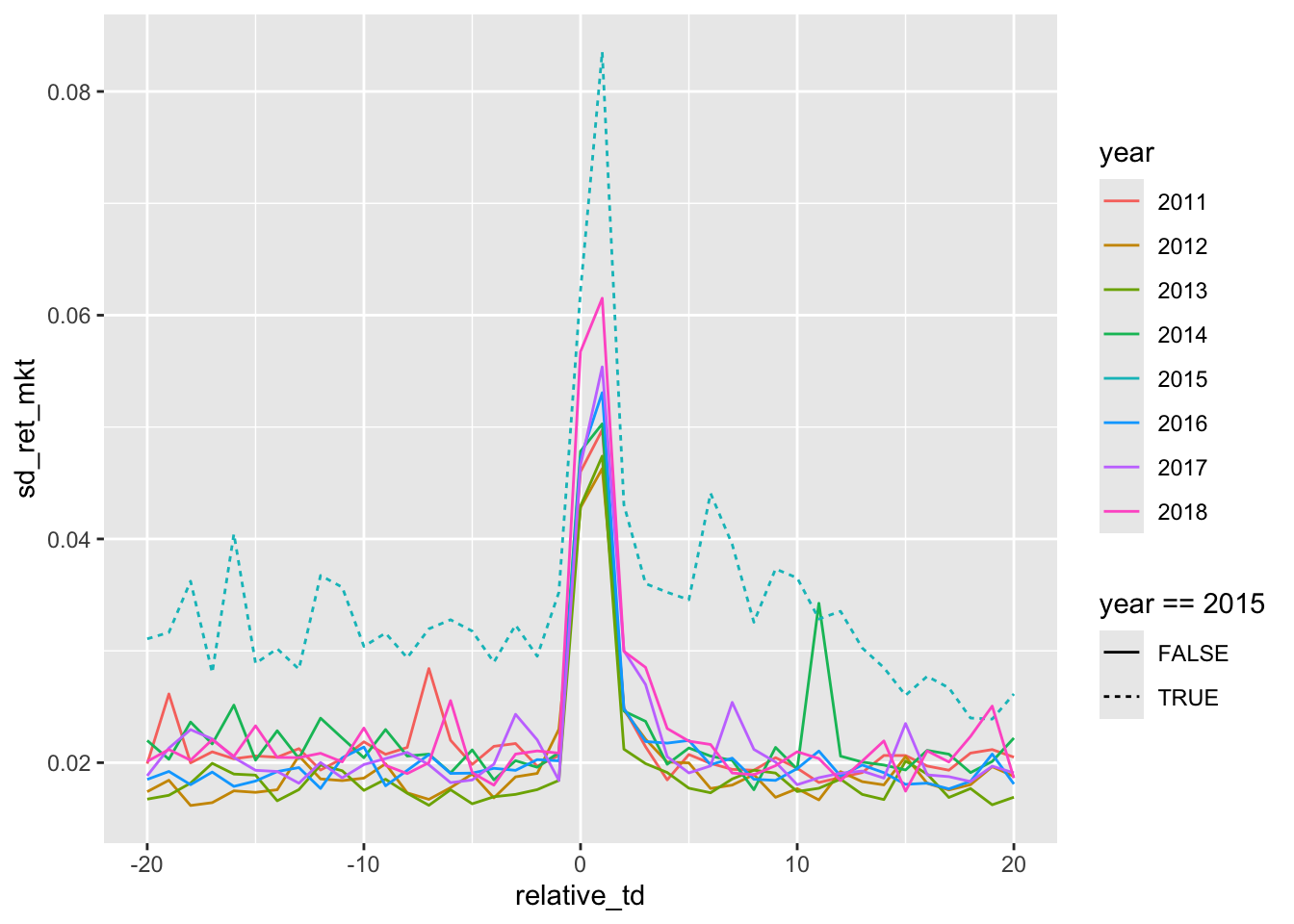
            .groups = "drop")

Now we can produce two plots. First, in Figure 12.2 we plot a measure of the standard deviation of market-adjusted returns. Each line represents a different year. The lines are largely indistinguishable from each other with the exception of 2015, which has high volatility throughout.

earn_annc_summ |>
  filter(year > 2010, year < 2019) |>
  mutate(year = as.factor(year)) |>
  ggplot(aes(x = relative_td, y = sd_ret_mkt,
             group = year, colour = year,
             linetype = year == 2015)) +
  geom_line()

Figure 12.2: Residual return volatility around earnings announcements

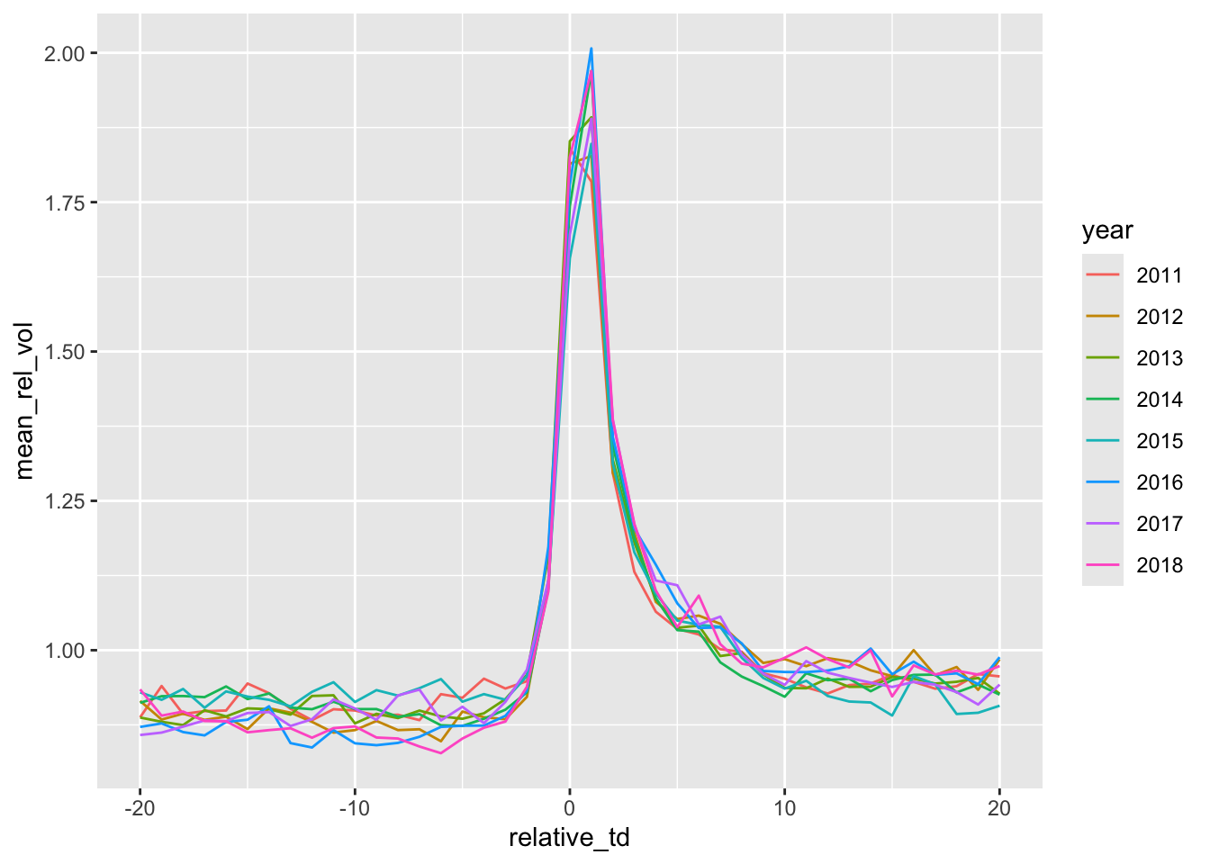
Second, in Figure 12.3 we plot a measure of the relative trading volumes.

earn_annc_summ |>
  filter(year > 2010, year < 2019) |>
  mutate(year = as.factor(year)) |>
  ggplot(aes(x = relative_td, y = mean_rel_vol,
             group = year, color = year)) +
  geom_line()

Figure 12.3: Relative trading volume around earnings announcements

dbDisconnect(db)

12.3 Discussion questions

1. After reading Bamber et al. (2000), do the reasons given by Beaver (1968) for his sample selection criteria still seem reasonable? Why or why not?

2. Bamber et al. (2000) do a replication and an extension of Beaver (1968). Why was it important to include the replication? What alternative approaches to extension could Bamber et al. (2000) have considered? Does it make sense to limit extensions to the sample period, available data, and methods of Beaver (1968)? What do you think of the claim that “the first research bricks (i.e., Beaver, 1968) affect the whole wall [of accounting research]”?

3. What’s the basic conclusion from the plots above in terms of whether “earnings announcements convey new information to the market”? Do the results support the conclusions made by subsequent researchers based on Beaver (1968)? Or do the concerns of Bamber et al. (2000) remain applicable?

4. In our replication analysis above, we made a number of measurement and design choices that differed from those made by Beaver (1968). What are those differences? Do you expect these to materially affect the tenor of the results? Do the choices we made seem appropriate if we were writing a research paper?

5. The plots above use daily data (Beaver, 1968 used weekly data). Apart from more statistical power, do the daily plots provide novel insights in this case?

6. What does the variable mad_ret_mkt on the data frame earn_annc_summ represent? Do results look different if this variable is used? Does this address the first concern about research design that Bamber et al. (2000) raise? If not, can you suggest (and apply) and alternative measure?

7. In the plots above, two filters have been applied: year > 2010 and year < 2019). Does it make sense to remove one or the other of these filters? What do you observe if you remove one or both of these? Can you explain these observations?

Ball, R., Brown, P., 1968. An empirical evaluation of accounting income numbers. Journal of Accounting Research 6, 159–178. https://doi.org/10.2307/2490232

Ball, R., Shivakumar, L., 2008. How much new information is there in earnings? Journal of Accounting Research 46, 975–1016. https://doi.org/10.1111/j.1475-679X.2008.00299.x

Bamber, L.S., Christensen, T.E., Gaver, K.M., 2000. Do we really “know” what we think we know? A case study of seminal research and its subsequent overgeneralization. Accounting, Organizations and Society 25, 103–129. https://doi.org/10.1016/S0361-3682(99)00027-6

Beaver, W.H., 1968. The information content of annual earnings announcements. Journal of Accounting Research 6, 67–92. https://doi.org/10.2307/2490070

Dechow, P.M., Sloan, R.G., Zha, J., 2014. Stock prices and earnings: A history of research. Annual Review of Financial Economics 6, 343–363. https://doi.org/10.1146/annurev-financial-110613-034522

---

1. As pointed out by Dechow et al. (2014), quarterly earnings announcements were not required during the sample period of Beaver (1968).

2. We will demonstrate shortly how we actually use this table.

3. As can be seen here, this function was added to dbplyr after a request related to creation of this course.

4. The variable exchcd is a header variable, meaning that there is one value for each PERMNO, even if a stock has traded on different exchanges over time. In Section 19.2.1, we are more careful and obtain the exchange on which a stock was traded on the relevant dates, but for our simple replication analysis here we ignore this detail.