6 Financial statements: A first look
This is the published R edition of the book. A Python version of the book is available at era_pl_book.
In this chapter, we provide an introduction to data on financial statements, which are the primary focus of financial reporting. While a lot of contemporary accounting research has only a tangential connection to financial reporting, it’s not clear there would be a field of accounting research without financial reporting and most accounting research papers use financial reporting data to some degree (e.g., as controls). In this chapter, we will focus on annual financial statement data of North American firms, as provided by Compustat.
In this chapter, we will use four R libraries. We have seen dplyr, ggplot2, and farr in earlier chapters, but the DBI library is new. The DBI library provides a standardized interface to relational database systems, including PostgreSQL (the system used by WRDS), MySQL, and SQLite. For instructions on how to set up your computer to use the code found in this book, see Section 1.2. Quarto templates for the exercises below are available on GitHub.
6.1 Setting up WRDS
Academic researchers generally get Compustat data through Wharton Research Data Services, more commonly referred to as WRDS (pronounced “words”). In the following, we assume that you have run the code above, that you have a WRDS account, and that you are connected to the internet.
Now let’s connect to the WRDS database. To actually use the code below, you should replace your_WRDS_ID with your actual WRDS ID. You may also need to add a line Sys.setenv(PGPASSWORD = "your_password") as the third line of code.1
Sys.setenv(PGHOST = "wrds-pgdata.wharton.upenn.edu",
           PGPORT = 9737L,
           PGUSER = "your_WRDS_ID",
           PGDATABASE = "wrds")

db <- dbConnect(RPostgres::Postgres(), bigint = "integer")
Academic researchers generally get Compustat data through Wharton Research Data Services, more commonly referred to as WRDS (pronounced “words”). In the following, we assume that you have created a local parquet library as described in Section E.6. To actually use the code below, you should replace the value set for DATA_DIR with the location of the data repository on your computer.
Sys.setenv(DATA_DIR = "~/Dropbox/pq_data")

db <- dbConnect(duckdb::duckdb())
The first line of code above sets up environment variables containing information that R can use as defaults when connecting to a PostgreSQL database. The second line of code creates the actual connection to the database and assigns it to the variable db. We set bigint = "integer" here because some packages cannot handle 64-bit integers of PostgreSQL’s bigint type, so we ask these to be mapped to the 32-bit integers used in R.2 We can also set check_interrupts = TRUE if we are running queries that take a long time so that we can interrupt them if we think something has gone wrong. Most queries in this book execute quickly, so this is generally not necessary.3
For users of the PostgreSQL database, an alternative to the code above would pass connection information to the dbConnect() function directly, as shown in the code below.4
However, we recommend using the environment variable-based approach above. We also recommend using the approach based on a .pgpass file discussed in detail in the WRDS instructions.5 Putting the connection details outside your code (e.g., in environment variables) makes it possible to write code that works both for you and for others, including your co-authors.
Now that we have established a connection to the WRDS data, we can get some data. Data sources on WRDS are organized into libraries according to their source (in PostgreSQL, these libraries are called schemas, but we will stick with the WRDS terminology for now).
In this chapter we focus on Compustat data, which is found in the comp library. While there are other sources of financial statement data—especially for firms outside North America—in accounting research the pre-eminent data source is Compustat, which is typically obtained via WRDS.
We first look at the table, comp.company, which contains information about the companies in Compustat’s North American database (the equivalent table in Compustat’s “Global” database is comp.g_company). By running the following code, we create R objects that point to the data on the WRDS database and behave a lot like the data frames you have seen in earlier chapters.
company <- load_parquet(db, schema = "comp", table = "company")What have we done here? In the first line, we have created an object company that “points to” the table company in schema comp in the data source db (which represents the connection to the database). From the help for the tbl() function, we learn that in tbl(src, ...), src refers to the data source. Here db is an object representing the connection to the WRDS PostgreSQL database. The ... allows us to pass other arguments to the function, and we pass Id(schema = "comp", table = "company") to indicate the underlying database object we are looking for.
But what exactly is company? One way to get information about company is to use the class() function.6
class(company)[1] "tbl_PqConnection" "tbl_dbi" "tbl_sql" "tbl_lazy"
[5] "tbl" The output here is a little complicated for a new user, but the basic idea is that company is a tbl_PqConnection object, and also a tbl_sql object and a tbl object, which means it a tibble of some kind. The critical idea here is that funda is a tbl_sql object, which means it behaves like a tibble, but is actually effectively a reference to a table or query in a relational database. For want of a better term, company is a remote data frame.
While there are some technical details here that are unimportant for our discussion, the important points are that, as a tbl_sql, funda has three important properties:
- It’s not a data frame in memory in R. This means that we don’t need to download all of the data and load it into R.
- It’s not a data frame in memory in the database (in this case, the remote WRDS PostgreSQL server). This means that we don’t load the full data set into memory even on the remote computer.
- Notwithstanding the previous two points,
companybehaves in many important ways just like a data frame.
We can use filter() to get only rows meeting certain conditions and we can use select() to indicate which columns we want to retrieve:
# Source: SQL [?? x 3]
# Database: postgres [igow@localhost:5432/igow]
gvkey conm state
<chr> <chr> <chr>
1 001690 APPLE INC CA
2 001820 ASTRONOVA INC RI
3 027925 AVID TECHNOLOGY INC MA
4 063446 AINOS INC CA
5 324055 ADVANCETC LTD <NA> When we are dealing with a remote data frame, the dplyr code that we write is automatically translated into SQL, a specialized language for manipulating tabular data “used by pretty much every database in existence” (Appendix B has more on SQL and dplyr).
We can inspect the translated SQL using show_query():
company |>
  filter(gsubind == "45202030",
         str_sub(conm, 1, 1) == "A") |>
  select(gvkey, conm, state) |>
head(5) |>
show_query()<SQL>
SELECT "gvkey", "conm", "state"
FROM "comp"."company"
WHERE ("gsubind" = '45202030') AND (SUBSTR("conm", 1, 1) = 'A')
LIMIT 5Here we see that filter() is translated into equivalent SQL using WHERE.
While remote data frames behave a lot like local data frames, they are not quite the same thing and, for many purposes, we need to use local data frames. For example, the lm() function for fitting regressions assumes that the object provided as its data argument is a data frame and it will not work if we give it a remote data frame instead. Conversion of a table from a remote data frame to a local one is achieved using the collect() verb. Here we use collect() and store the result in df_company.
Looking at class(df_company), we see that it is not only a “tibble” (tbl_df), but also data.frame, meaning that we can pass it to functions (such as lm()) that expect data.frame objects.
class(df_company)[1] "tbl_df" "tbl" "data.frame"df_company# A tibble: 5 × 3
gvkey conm state
<chr> <chr> <chr>
1 001690 APPLE INC CA
2 001820 ASTRONOVA INC RI
3 027925 AVID TECHNOLOGY INC MA
4 063446 AINOS INC CA
5 324055 ADVANCETC LTD <NA> 6.2 Financial statement data
Two core tables for the North American Compustat data are comp.funda, which contains annual financial statement data, and comp.fundq, which contains quarterly data.
fundq <- load_parquet(db, schema = "comp", table = "fundq")
funda <- load_parquet(db, schema = "comp", table = "funda")
We can examine the first object in R by typing its name in the R console:
funda# Source: table<"comp"."funda"> [?? x 949]
# Database: postgres [igow@localhost:5432/igow]
gvkey datadate fyear indfmt consol popsrc datafmt tic cusip conm
<chr> <date> <int> <chr> <chr> <chr> <chr> <chr> <chr> <chr>
1 001017 1979-02-28 1978 INDL C D STD AELNA 00103… AEL …
2 001017 1980-02-29 1979 INDL C D STD AELNA 00103… AEL …
3 001017 1981-02-28 1980 INDL C D STD AELNA 00103… AEL …
4 001017 1982-02-28 1981 INDL C D STD AELNA 00103… AEL …
5 001017 1983-02-28 1982 INDL C D STD AELNA 00103… AEL …
6 001084 1979-09-30 1979 INDL C D STD WDDD 98159… WORL…
7 001017 1984-02-29 1983 INDL C D STD AELNA 00103… AEL …
8 001017 1985-02-28 1984 INDL C D STD AELNA 00103… AEL …
9 001017 1986-02-28 1985 INDL C D STD AELNA 00103… AEL …
10 001017 1986-02-28 1985 INDL C D SUMM_STD AELNA 00103… AEL …
# ℹ more rows
# ℹ 939 more variables: acctchg <chr>, acctstd <chr>, acqmeth <chr>,
# adrr <dbl>, ajex <dbl>, ajp <dbl>, bspr <chr>, compst <chr>,
# curcd <chr>, curncd <chr>, currtr <dbl>, curuscn <dbl>, final <chr>,
# fyr <int>, ismod <int>, ltcm <chr>, ogm <chr>, pddur <int>, scf <int>,
# src <int>, stalt <chr>, udpl <chr>, upd <int>, apdedate <date>,
# fdate <date>, pdate <date>, acchg <dbl>, acco <dbl>, accrt <dbl>, …From this code, we can see that comp.funda is a very wide table, with 949 columns. With so many columns, it’s a moderately large table (at the time of writing, 1212 MB in PostgreSQL), but by focusing on certain columns, the size of the data can be dramatically reduced. Let’s learn more about this table.
First, how many rows does it have?
From this snippet, we can see that comp.funda has 935,204 rows. When given an ungrouped data frame as the first argument, the count() function simply counts the number of rows in the data frame.7 In this case, funda |> count() returns a server-side data frame with a single column (n). The command pull() extracts that single column as a vector in R.8
While not evident from casual inspection of the table, the primary key of comp.funda is (gvkey, datadate, indfmt, consol, popsrc, datafmt). One requirement for a valid primary key is that each value of the primary key is associated with only one row of the data set. (Chapter 19 of R for Data Science discusses this point.) That this requirement is met can be seen with output from the following code, which counts the number of rows associated with each set of values for (gvkey, datadate, indfmt, consol, popsrc, datafmt) and stores that number in num_rows and then displays the various values of num_rows.
# A tibble: 935,204 × 7
   gvkey  datadate   indfmt consol popsrc datafmt  num_rows
   <chr>  <date>     <chr>  <chr>  <chr>  <chr>       <int>
 1 001107 1995-12-31 INDL   C      D      STD             1
 2 003969 2003-12-31 INDL   C      D      SUMM_STD        1
 3 003570 2002-07-31 INDL   C      D      SUMM_STD        1
 4 001567 1962-12-31 INDL   C      D      STD             1
 5 001537 1972-12-31 INDL   C      D      STD             1
 6 001026 1976-12-31 INDL   C      D      STD             1
 7 001078 2010-12-31 INDL   C      D      STD             1
 8 003205 1982-12-31 INDL   C      D      STD             1
 9 003818 1966-12-31 INDL   C      D      STD             1
10 002275 1985-09-30 INDL   C      D      SUMM_STD        1
# ℹ 935,194 more rows
Because num_rows is equal to 1 in 935,204 cases and this is the number of rows in the data set, we have (gvkey, datadate, indfmt, consol, popsrc, datafmt) as a valid key.
The second requirement of a primary key is that none of the columns contains null values (in SQL, NULL; in R, NA). The code below checks this.
[1] 0Teasing apart the primary key, we have a firm identifier (gvkey) and financial period identifier (datadate), along with four variables that are more technical in nature: indfmt, consol, popsrc, and datafmt. Table 6.1 provides the number of observations for each set of values of these four variables.
(indfmt, consol, popsrc, datafmt) values
| indfmt | consol | popsrc | datafmt | n |
|---|---|---|---|---|
| INDL | C | D | STD | 596,500 |
| INDL | C | D | SUMM_STD | 288,157 |
| FS | C | D | STD | 48,424 |
| INDL | P | D | STD | 1,179 |
| INDL | R | D | STD | 480 |
| INDL | P | D | SUMM_STD | 306 |
| FS | R | D | STD | 51 |
| INDL | R | D | SUMM_STD | 28 |
| INDL | D | D | SUMM_STD | 25 |
| INDL | D | D | STD | 25 |
| INDL | C | D | PRE_AMENDS | 19 |
| INDL | C | D | PRE_AMENDSS | 10 |
As discussed on the CRSP website, the first set of values, which covers 596,500 observations, represents the standard (STD) secondary keyset, as it is what is used by most researchers when using Compustat. We can create a version of funda that limits data to this STD secondary keyset as follows:
funda_mod <-
  funda |>
  filter(indfmt == "INDL", datafmt == "STD",
         consol == "C", popsrc == "D")
For funda_mod, (gvkey, datadate) should represent a primary key. We can check the first requirement using code like that we used above (we already confirmed the second requirement for the larger data set).
# A tibble: 1 × 2
  num_rows      n
     <int>  <int>
1        1 596500
Now, let’s look at the table comp.company, which the following code confirms has 40 columns and for which gvkey is a primary key.
company# Source: table<"comp"."company"> [?? x 40]
# Database: postgres [igow@localhost:5432/igow]
conm gvkey add1 add2 add3 add4 addzip busdesc cik city conml
<chr> <chr> <chr> <chr> <chr> <chr> <chr> <chr> <chr> <chr> <chr>
1 A & E PL… 0010… <NA> <NA> <NA> <NA> <NA> A & E … <NA> <NA> A & …
2 A & M FO… 0010… 1924… <NA> <NA> <NA> 94104 <NA> 0000… Tulsa A & …
3 AAI CORP 0010… 124 … <NA> <NA> <NA> 21030… Textro… 0001… Hunt… AAI …
4 A.A. IMP… 0010… 7700… <NA> <NA> <NA> 63125 A.A. I… 0000… St. … A.A.…
5 AAR CORP 0010… One … <NA> <NA> <NA> 60191 AAR Co… 0000… Wood… AAR …
6 A.B.A. I… 0010… 1026… <NA> <NA> <NA> 33782 A.B.A.… <NA> Pine… A.B.…
7 ABC INDS… 0010… 301 … <NA> <NA> <NA> 46590 ABC In… <NA> Wino… ABC …
8 ABKCO IN… 0010… 1700… <NA> <NA> <NA> 10019 ABKCO … 0000… New … ABKC…
9 ABM COMP… 0010… 3 Wh… <NA> <NA> <NA> 92714 ABM Co… <NA> Irvi… ABM …
10 ABS INDU… 0010… Inte… <NA> <NA> <NA> 44904 ABS In… 0000… Will… ABS …
# ℹ more rows
# ℹ 29 more variables: costat <chr>, county <chr>, dlrsn <chr>, ein <chr>,
# fax <chr>, fic <chr>, fyrc <int>, ggroup <chr>, gind <chr>,
# gsector <chr>, gsubind <chr>, idbflag <chr>, incorp <chr>, loc <chr>,
# naics <chr>, phone <chr>, prican <chr>, prirow <chr>, priusa <chr>,
# sic <chr>, spcindcd <int>, spcseccd <int>, spcsrc <chr>, state <chr>,
# stko <int>, weburl <chr>, dldte <date>, ipodate <date>, …First, each gvkey value is associated with just one row.
# A tibble: 1 × 2
  num_rows     n
     <int> <int>
1        1 56754
Second, there are no missing values of gvkey.
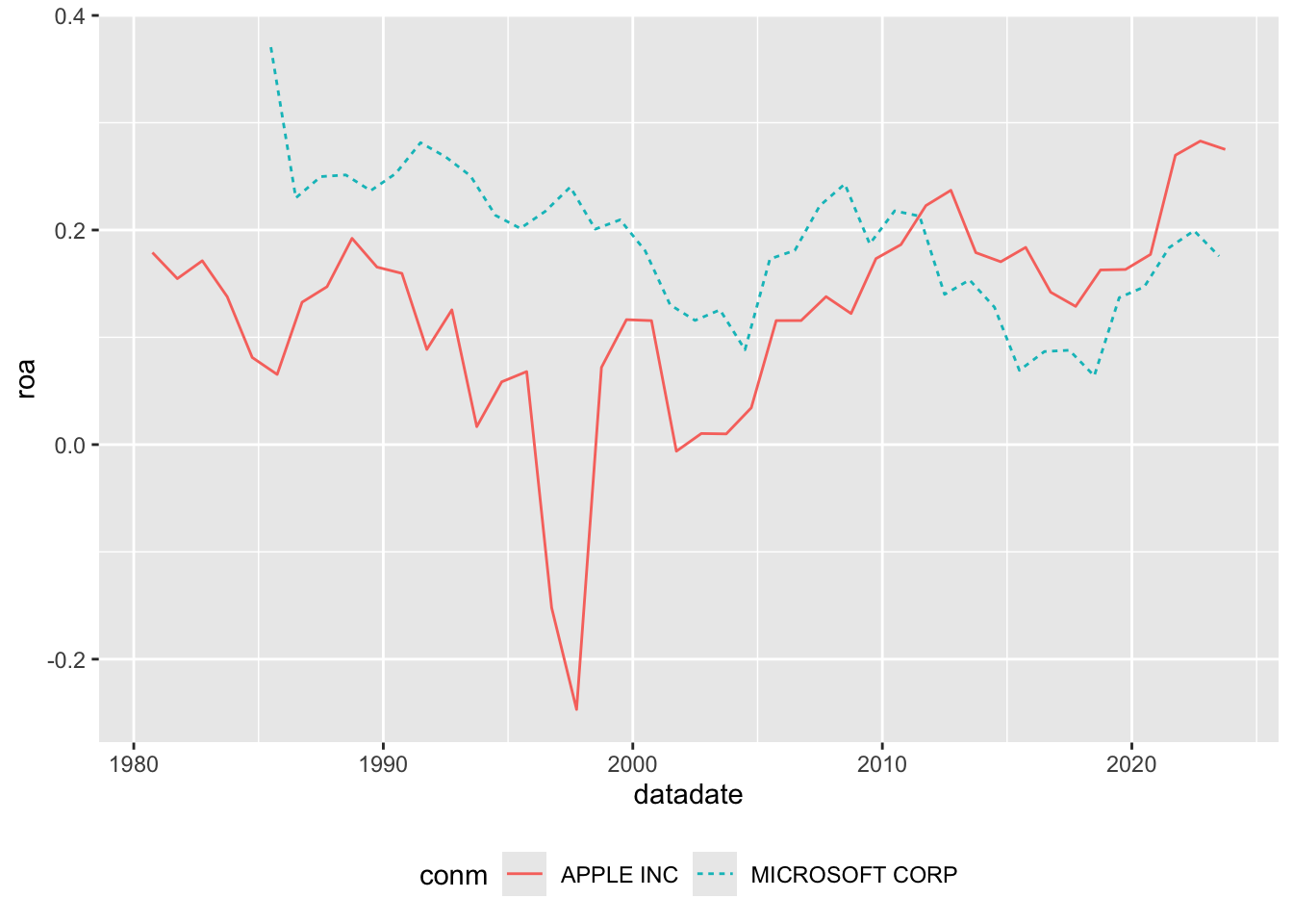
6.2.1 Illustration: Microsoft versus Apple
Suppose that we were interested in comparing the profitability of Apple and Microsoft over time. To measure performance, we will calculate a measure of return on assets, here measured as the value of “Income Before Extraordinary Items” scaled by “Total Assets” for Microsoft (GVKEY: 012141) and Apple (GVKEY: 001690) over time.9
# Source:   SQL [?? x 2]
# Database: postgres  [igow@localhost:5432/igow]
  conm           gvkey
  <chr>          <chr>
1 APPLE INC      001690
2 MICROSOFT CORP 012141
Here we can see that sample is a server-side data frame with the company name (conm) and identifier (gvkey) for Apple and Microsoft. We can use show_query() to see what the server-side data frame represents.
sample |>
  show_query()
<SQL>
SELECT "conm", "gvkey"
FROM "comp"."company"
WHERE ("gvkey" IN ('001690', '012141'))Here filter() is translated into a WHERE condition, %in% is translated to IN, and c("001690", "012141") is translated to ('001690', '012141').
It turns out that “Income Before Extraordinary Items” is represented by ib and “Total Assets” is at (see the CRSP manual for details). We can further restrict funda beyond funda_mod so that it contains just the key variables (gvkey, datadate) and the values for ib and at as follows. (In the following code, we will gradually refine the data set assigned to ib_at.)
# Source:   SQL [?? x 4]
# Database: postgres  [igow@localhost:5432/igow]
  gvkey  datadate       ib    at
  <chr>  <date>      <dbl> <dbl>
1 001017 1979-02-28  2.00   43.9
2 001017 1980-02-29 -0.177  53.5
3 001017 1981-02-28  0.478  54.0
4 001017 1982-02-28 -4.72   60.2
5 001017 1983-02-28  2.24   47.3
and then restrict this by joining it with sample as follows:
ib_at <-
  funda_mod |>
  select(gvkey, datadate, ib, at) |>
  inner_join(sample)
Joining with `by = join_by(gvkey)`ib_at |> head(5)# Source: SQL [?? x 5]
# Database: postgres [igow@localhost:5432/igow]
gvkey datadate ib at conm
<chr> <date> <dbl> <dbl> <chr>
1 001690 1980-09-30 11.7 65.4 APPLE INC
2 001690 1981-09-30 39.4 255. APPLE INC
3 001690 1982-09-30 61.3 358. APPLE INC
4 001690 1983-09-30 76.7 557. APPLE INC
5 001690 1984-09-30 64.1 789. APPLE INCIn the code above, we used a natural join, which joins by variables found in both data sets (in this case, gvkey). In general, we want to be explicit about the join variables, which we can do using the by argument to the join function:
ib_at <-
  funda_mod |>
  select(gvkey, datadate, ib, at) |>
  inner_join(sample, by = "gvkey")

ib_at |> head(5)
# Source: SQL [?? x 5]
# Database: postgres [igow@localhost:5432/igow]
gvkey datadate ib at conm
<chr> <date> <dbl> <dbl> <chr>
1 001690 2025-09-30 112010 359241 APPLE INC
2 012141 1985-06-30 24.1 65.1 MICROSOFT CORP
3 001690 1980-09-30 11.7 65.4 APPLE INC
4 001690 1981-09-30 39.4 255. APPLE INC
5 001690 1982-09-30 61.3 358. APPLE INC We next calculate a value for return on assets (using income before extraordinary items and the ending balance of total assets for simplicity).
ib_at <-
  funda_mod |>
  select(gvkey, datadate, ib, at) |>
  inner_join(sample, by = "gvkey") |>
  mutate(roa = ib / at)
The final step is to bring these data into R. At this stage, ib_at is still a server-side data frame (tbl_sql), which we can see using the class function.10
To bring the data into R, we can use the collect() function, as follows:
ib_at <-
  funda_mod |>
  select(gvkey, datadate, ib, at) |>
  inner_join(sample, by = "gvkey") |>
  mutate(roa = ib / at) |>
  collect()
Now we have a local data frame that is no longer an instance of the tbl_sql class:
class(ib_at)[1] "tbl_df" "tbl" "data.frame"Note that because we have used select() to get to just five fields and filter() to focus on two firms, the tibble ib_at is just 6.1 kB in size. Note the placement of collect() at the end of this pipeline means that the amount of data we need to retrieve from the database and load into R is quite small. If we had placed collect() immediately after funda_mod, we would have been retrieving data on thousands of observations and 949 variables. If we had placed collect() immediately after the select() statement, we would have been retrieving data on thousands of observations, but just 4 variables. But by placing collect() after the inner_join(), we are only retrieving data for firm-years related to Microsoft and Apple. Retrieving data into our local R instance requires both reading it off disk and, if our database server is remote, transferring it over the internet. Each of these operations is (relatively) slow and thus should be avoided where possible.
Having collected our data, we can make Figure 6.1.11
6.3 Exercises
Suppose we didn’t have access to Compustat (or an equivalent database) for the analysis above, describe a process you would use to get the data required to make the plot above comparing performance of Microsoft and Apple.
In the following code, how do
funda_modandfunda_mod_altdiffer? (For example, where are the data for each table?) What does the statementcollect(n = 100)at the end of this code do?
funda <- load_parquet(db, schema = "comp", table = "funda")

funda_mod <-
  funda |>
  filter(indfmt == "INDL", datafmt == "STD",
         consol == "C", popsrc == "D") |>
  filter(fyear >= 1980)

funda_mod_alt <-
  funda_mod |>
collect(n = 100)- The table
comp.companyhas data on SIC (Standard Industrial Classification) codes in the fieldsic. In words, what is thecase_when()function doing in the following code? Why do we end up with just two rows?
- What does the data frame
another_samplerepresent? What happens if we change theinner_join()below to simplyinner_join(sample)? What happens if we change it toinner_join(sample, by = "sic")(i.e., omit thesuffix = c("", "_other")portion)? Why do we usefilter(gvkey != gvkey_other)?
- What is the following code doing?
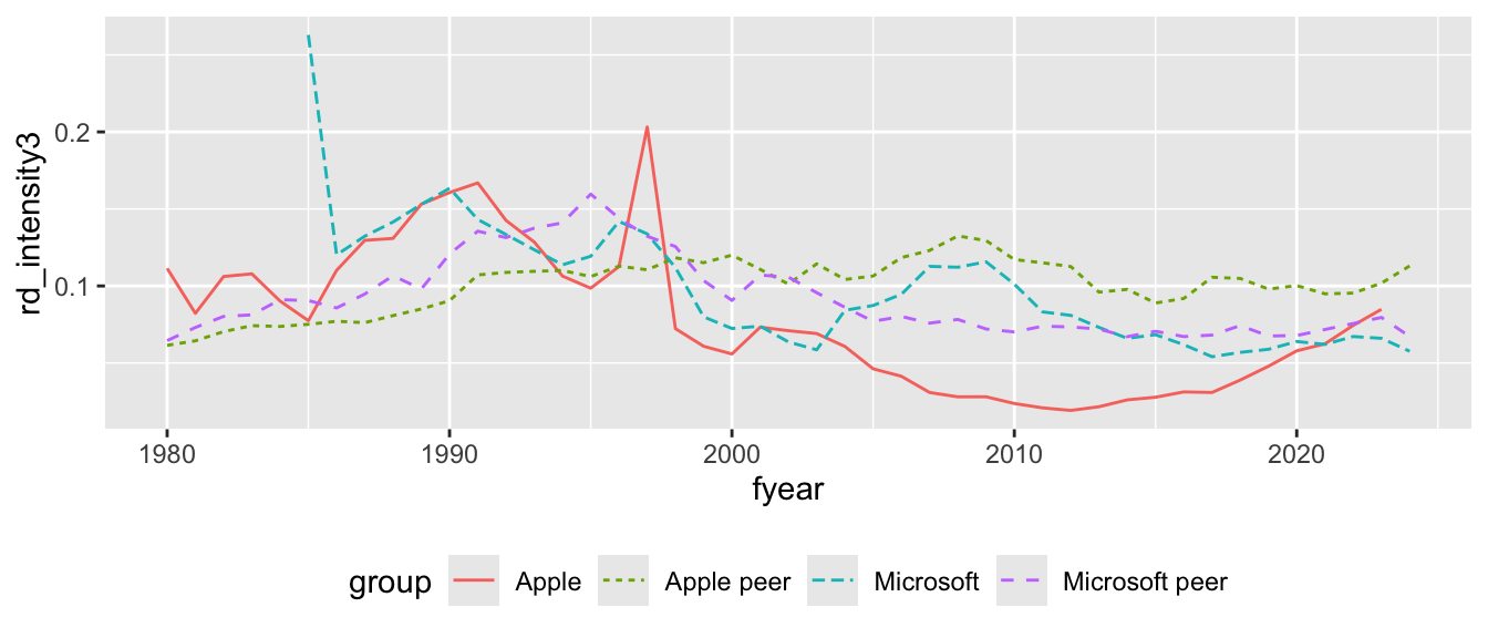
- Suppose that we are interested in firms’ R&D activity. One measure of R&D activity is R&D Intensity, which can be defined as “R&D expenses” (Compustat item
xrd) scaled by “Total Assets” (Compustat itemat). Inxrd_at, what’s the difference betweenrd_intensityandrd_intensity_alt? Doesfilter(at > 0)seem like a reasonable filter? What happens if we omit it?
xrd_at <-
  funda_mod |>
  select(gvkey, datadate, fyear, conm, xrd, at) |>
  filter(at > 0) |>
  mutate(rd_intensity = xrd / at,
         xrd_alt = coalesce(xrd, 0),
         rd_intensity_alt = xrd_alt / at) |>
inner_join(total_sample, by = "gvkey") - Looking at a sample of rows from
xrd_at_sum, it appears that the three R&D intensity measures are always identical for Apple and Microsoft, but generally different for their peer groups. What explains these differences? Can you say that one measure is “correct”? Or would you say “it depends”?
# A tibble: 8 × 5
  group          fyear rd_intensity1 rd_intensity2 rd_intensity3
  <chr>          <int>         <dbl>         <dbl>         <dbl>
1 Apple           2025        0.0962        0.0962        0.0962
2 Apple peer      2025        0.117         0.117         0.117
3 Microsoft       2025        0.0525        0.0525        0.0525
4 Microsoft peer  2025        0.132         0.114         0.0625
5 Apple           2024        0.0859        0.0859        0.0859
6 Apple peer      2024        0.136         0.132         0.119
7 Microsoft       2024        0.0576        0.0576        0.0576
8 Microsoft peer 2024 0.297 0.241 0.0705- Write code to produce Figure 6.2. Also produce plots that use
rd_intensity1andrd_intensity2as measures of R&D intensity. Do the plots help you think about which of the three measures makes most sense?
We put our passwords in a special password file, as described here, so we don’t need this step. It’s obviously not a good idea to put your password in code.↩︎
The data we use in this book will not exceed the limits of 32-bit integers, so this involves no loss. See the help for
RPostgresfor more information. You can access this help by typing? RPostgres::Postgresin the R console.↩︎We flag longer running queries when they arise.↩︎
Remove the
#from the lines beginning with#and replace the password and user name if you try this.↩︎See https://go.unimelb.edu.au/kv68. Note that we do not recommend setting up a connection to WRDS in your
.Rprofileas suggested by WRDS, as this yields code that is less transparent and usable by others. Additionally, it means setting up a connection even when you may not need one.↩︎If you are using the parquet file–based approach, your output will differ from what is shown here.↩︎
Many
dplyrfunctions take data frames as (first) arguments and return data frames as values.↩︎As that vector has a single value, it is displayed without any information about the database connection that we used to get the information. This looks cleaner in this setting, as you can see yourself if you run the command yourself without
pull()at the end.↩︎Financial analysts might object to using an end-of-period value as the denominator; we do so here because it simplifies the coding and our goal here is just illustrative.↩︎
An alternative to this line would be
inherits(ib_at, "tbl_sql"). More on classes can be found in “Advanced R” at https://adv-r.hadley.nz.↩︎Note that even if we hadn’t called
collect(), recent versions ofggplot2are aware of remote data frames and will take care of this for us. But other functions (e.g.,lm(), which we saw in Chapter 4) are not aware of remote data frames and thus require us to usecollect()before passing data to them.↩︎