import polars as pl
from plotnine import ggplot
from plotnine.data import mpgFacets (Subplots)
This notebook adapts the plotnine guide on facets to the fluent API style.
Setup
mpg = pl.from_pandas(mpg)
mpg.head()
shape: (5, 11)
| manufacturer | model | displ | year | cyl | trans | drv | cty | hwy | fl | class |
|---|---|---|---|---|---|---|---|---|---|---|
| str | str | f64 | i64 | i64 | str | str | i64 | i64 | str | str |
| "audi" | "a4" | 1.8 | 1999 | 4 | "auto(l5)" | "f" | 18 | 29 | "p" | "compact" |
| "audi" | "a4" | 1.8 | 1999 | 4 | "manual(m5)" | "f" | 21 | 29 | "p" | "compact" |
| "audi" | "a4" | 2.0 | 2008 | 4 | "manual(m6)" | "f" | 20 | 31 | "p" | "compact" |
| "audi" | "a4" | 2.0 | 2008 | 4 | "auto(av)" | "f" | 21 | 30 | "p" | "compact" |
| "audi" | "a4" | 2.8 | 1999 | 6 | "auto(l5)" | "f" | 16 | 26 | "p" | "compact" |
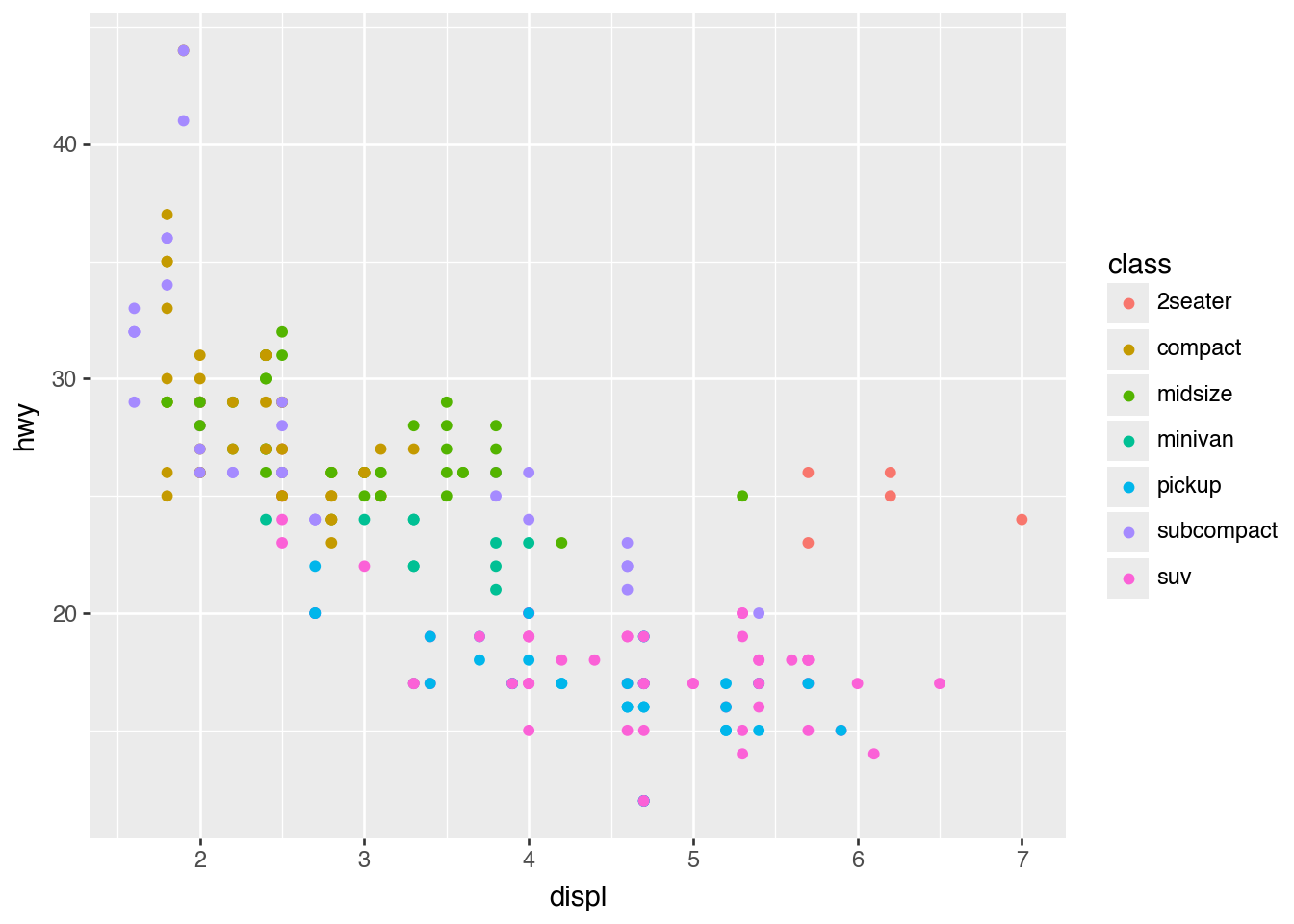
Here is a single large plot that we can split into subplots.
(
    ggplot(mpg)
    .aes("displ", "hwy", color="class")
    .geom_point()
)
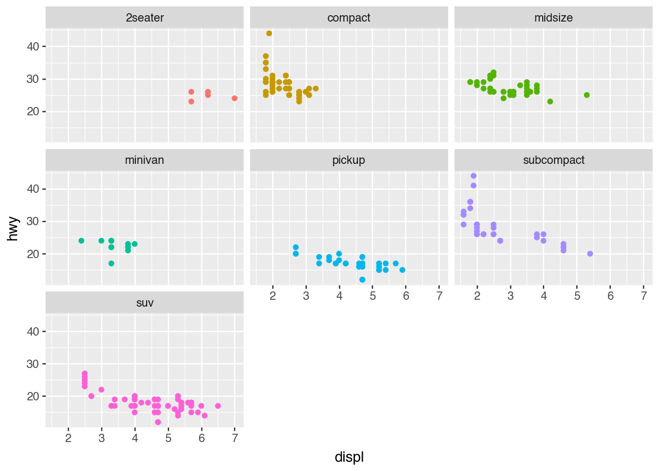
facet_wrap(): Subplot Sequence
(
    ggplot(mpg)
    .aes("displ", "hwy", color="class")
    .geom_point(show_legend=False)
    .facet_wrap("class")
)
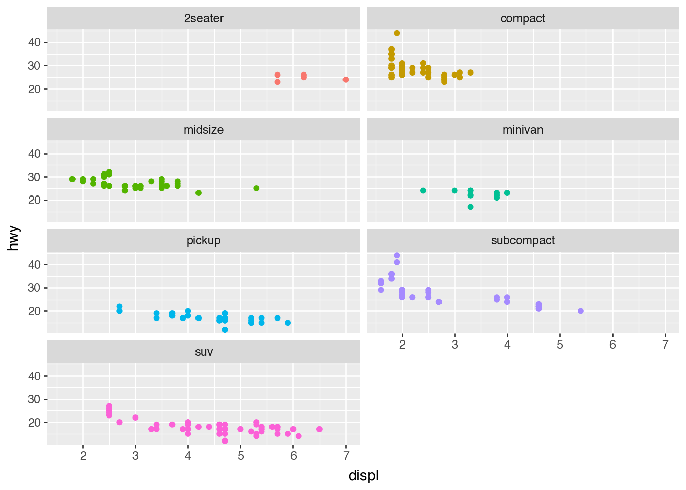
Use ncol= or nrow= to control the layout.
(
    ggplot(mpg)
    .aes("displ", "hwy", color="class")
    .geom_point(show_legend=False)
    .facet_wrap("class", ncol=2)
)
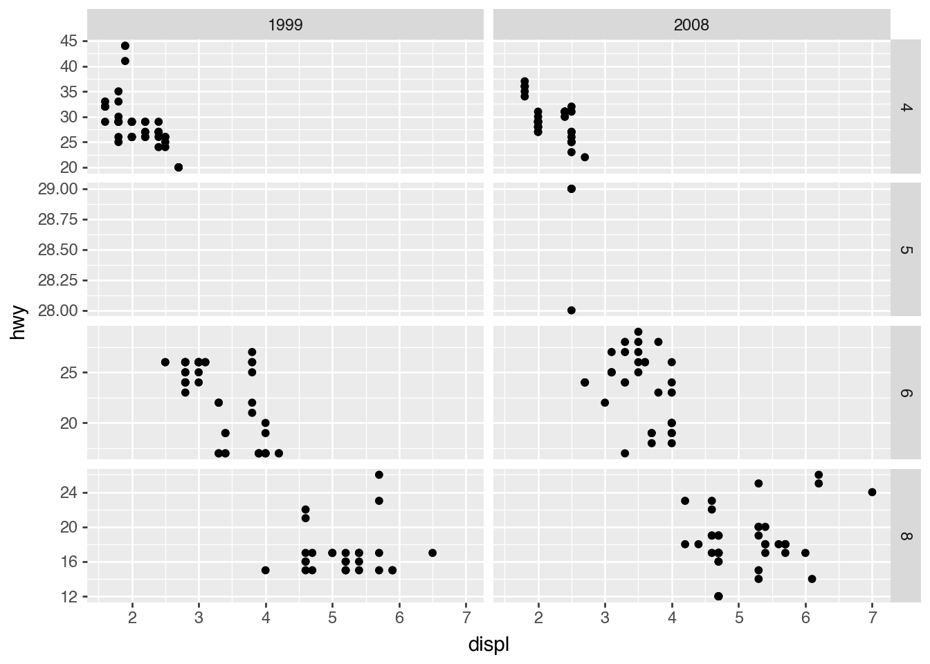
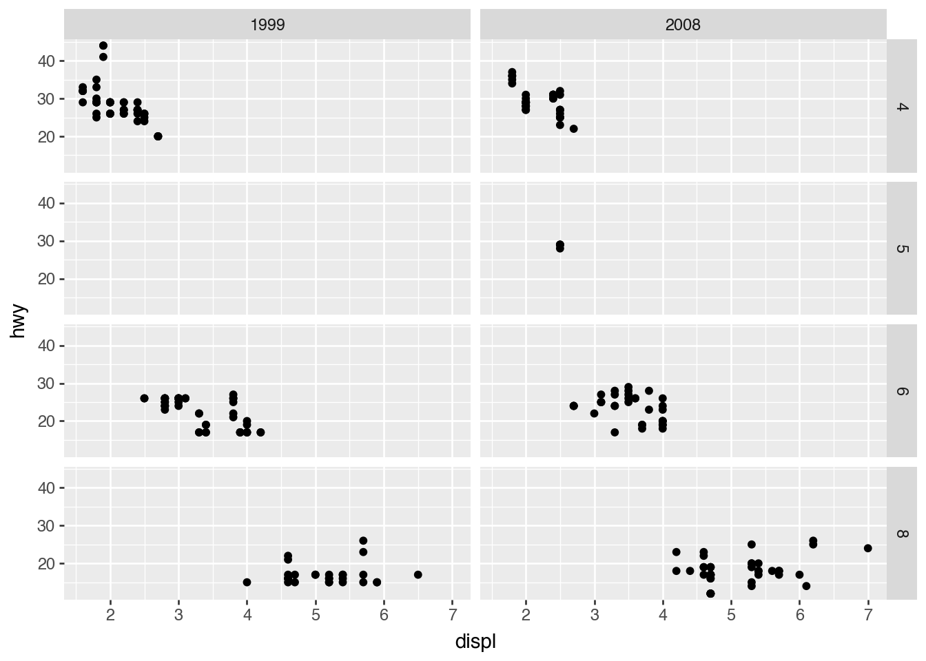
facet_grid(): Subplot Matrix
(
    ggplot(mpg)
    .aes("displ", "hwy")
    .geom_point()
    .facet_grid("cyl", "year")
)
Facetting Formula Syntax
Both facet_wrap() and facet_grid() support a formula-like syntax.
(
    ggplot(mpg)
    .aes("displ", "hwy")
    .geom_point()
    .facet_grid("cyl ~ year")
)
scales= for Freeing Axes
(
    ggplot(mpg)
    .aes("displ", "hwy")
    .geom_point()
    .facet_grid("cyl ~ year", scales="free_y")
)