import numpy as np
import polars as pl
from plotnine_polars import aes

import statsmodels.api as sm
import statsmodels.formula.api as smf
import pyfixest as pf

from maketables import ETable

from era_pl import load_data, ols_dropcollinear3 Regression fundamentals
In this chapter, we provide a short introduction to the fundamentals of regression analysis with a focus on ordinary least-squares (OLS) regression. Our emphasis here is on helping the reader to build intuition for the mechanics of regression. We demonstrate different ways of achieving various regression results to strengthen the reader’s intuition for what regression is doing. In this spirit, we close the chapter with a brief discussion of the Frisch-Waugh-Lovell theorem, which provides a way of representing multivariate regression coefficients as the result of a single-variable regression.
While we motivate some of our regressions with a data set that prompts a number of causal questions, we largely sidestep the issue of when OLS regression does or does not produce valid estimates of causal effects. Thus, while we hint at possible causal interpretations of results in this chapter, the reader should be cautious about these interpretations. We begin our formal analysis of causal inference with Chapter 4.
Additionally, while we note that OLS will provide noisy estimates of estimands, we do not address issues regarding how precise these estimates are or how to assess the statistical significance of results.1 A few p-values and t-statistics will crop up in regression analysis shown in this chapter, but we ignore those details for now. We begin our study of statistical inference in Chapter 5.
Tip
The code in this chapter uses the packages listed below. For instructions on how to set up your computer to use this code, go to the support page for this book. The support page also includes Quarto templates for the code and exercises below.
3.1 Introduction
Suppose we have data on variables \(y\), \(x_1\) and \(x_2\) for \(n\) units and we conjecture that there is a linear relationship between these variables of the following form:
\[ y_i = \beta_0 + \beta_1 \times x_{i1} + \beta_2 \times x_{i2} + \epsilon_i \] where \(i \in {1, \dots, n}\) denotes the data for a particular unit. We can write that in matrix form as follows:
\[ \begin{bmatrix} y_1 \\ y_2 \\ \dots \\ y_{n-1} \\ y_{n} \\ \end{bmatrix} = \begin{bmatrix} 1 & x_{11} & x_{12} \\ 1 & x_{21} & x_{22} \\ \dots & \dots & \dots \\ 1 & x_{n-1,1} & x_{n-1, 2} \\ 1 & x_{n, 1} & x_{n, 2} \end{bmatrix} \times \begin{bmatrix} \beta_0 \\ \beta_1 \\ \beta_2 \end{bmatrix} + \begin{bmatrix} \epsilon_1 \\ \epsilon_2 \\ \dots \\ \epsilon_{n-1} \\ \epsilon_{n} \\ \end{bmatrix} \]
And this can be written even more compactly as:
\[ y = X \beta + \epsilon \] where \(X\) is an \(n \times 3\) matrix and \(y\) is an \(n\)-element vector. It is conventional to denote the number of columns in the \(X\) matrix using \(k\), where \(k = 3\) in this case.2
In a regression context, we call \(X\) the regressors, \(y\) the regressand, and \(\epsilon\) the error term. We assume that we observe \(X\) and \(y\), but not \(\epsilon\). If we did observe \(\epsilon\), then we could probably solve for the exact value of the coefficients \(\beta\) with just a few observations. Lacking such information, we can produce an estimate of our estimand, \(\beta\). Our estimate (\(\hat{\beta}\)) is likely to differ from \(\beta\) due to noise arising from the randomness of the unobserved \(\epsilon\) and also possibly bias. There will usually be a number of estimators that we might consider for a particular problem. We will focus on the ordinary least-squares regression (or OLS) estimator as the source for our estimates in this chapter.
OLS is a mainstay of empirical research in the social sciences in general and in financial accounting in particular. In matrix notation, the OLS estimator is given by
\[ \hat{\beta} = (X^{\mathsf{T}}X)^{-1}X^{\mathsf{T}}y \]
Let’s break this down. First, \(X^{\mathsf{T}}\) is the transpose of \(X\), meaning the \(k \times n\) matrix formed by making the rows of \(X\) into columns. Second, \(X^{\mathsf{T}} X\) is the product of the \(k \times n\) matrix \(X^{\mathsf{T}}\) and the \(n \times k\) matrix \(X\), which results in a \(k \times k\) matrix. Third, the \(-1\) exponent indicates the inverse matrix. For a real number \(x\), \(x^{-1}\) denotes the number that when multiplied by \(x\) gives \(1\) (i.e., \(x \times x^{-1} = 1\)). For a square matrix \(Z\) (here “square” means the number of rows equals the number of columns), \(Z^{-1}\) denotes the square matrix that when multiplied by \(Z\) gives the identity matrix, \(\mathbf{I}\) (i.e., \(Z \times Z^{-1} = \mathbf{I}\)).
The \(3 \times 3\) identity matrix looks like this
\[ \begin{bmatrix} 1 & 0 & 0 \\ 0 & 1 & 0 \\ 0 & 0 & 1 \end{bmatrix} \]
Note that, just as there is no meaningful way to calculate the inverse of \(0\), it’s not always possible to take the inverse of a matrix. But, so long as no column of \(X\) is a linear combination of other columns and \(n > k\), then we can calculate \((X^{\mathsf{T}}X)^{-1}\) (and there are standard algorithms for doing so). Now, \(X^{\mathsf{T}}y\) is the product of a \(k \times n\) matrix (\(X^{\mathsf{T}}\)) and a vector with \(n\) elements (this can be thought of as an \(n \times 1\) matrix), so the result will be a \(k \times 1\) matrix. Thus, the product of \((X^{\mathsf{T}}X)^{-1}\) and \(X^{\mathsf{T}}y\) will be a vector with \(k\) elements, which we can denote as follows:
\[ \begin{bmatrix} \hat{\beta}_1 \\ \hat{\beta}_2 \\ \hat{\beta}_3 \\ \end{bmatrix} \]
So \(X^{\mathsf{T}}X\) is a \(k \times k\) matrix (as is its inverse), and \(X^{\mathsf{T}}y\) is the product of a \(k \times N\) matrix times an \(N \times 1\) matrix (i.e., a vector). So \(\hat{\beta}\) is a \(k\)-element vector. If we have a single regressor \(x\), then \(X\) will typically include the constant term, so \(k = 2\).
For this chapter, we will assume that the model \(y = X \beta + \epsilon\) is a structural (causal) model. What this means is that if we could somehow increase the value of \(x_{i1}\) by 1 unit without changing any other part of the system, we would see an increase in the value of \(y_{i}\) equal to \(\beta_1\). This model is causal in the sense that a unit change in \(x_{i1}\) can be said to cause a \(\beta_1\) change in \(y_i\).
rng = np.random.default_rng(2021)
N   = 1000
x1 = rng.standard_normal(N)
x2 = rng.standard_normal(N)
e  = rng.normal(0, 0.2, N)
y  = 1.0 * x1 + 2.0 * x2 + e
To make this more concrete, let’s consider some actual (though not “real”) data. The code above uses NumPy’s random-number generator to create simulated data. Specifically, we generate 1000 observations with \(\beta = 1\) and \(\sigma = 0.2\). This is the first of at least a dozen simulation analyses that we will consider in the book.
To make our analysis easier to replicate, we include np.random.default_rng(2021) to set the random-number generator used by rng.standard_normal() to the same point, so that we can reproduce the analysis ourselves later and so that others can reproduce it too. For a beginner-friendly introduction to random-number generation in NumPy, see the Random sampling documentation. Note that the value 2021 is arbitrary and represents nothing more than the year in which this material was first written. Any value would work here, e.g., 2024, 42, or 20240215 could be used.
We next construct \(X\) as a matrix comprising a column of ones (to estimate the constant term) and a column containing \(x\).
X = np.column_stack([np.ones(N), x1, x2])
X[:6]
array([[ 1. , -0.0688612 , 0.03089403],
[ 1. , -0.68696559, -0.46641998],
[ 1. , -0.7884868 , 0.96300525],
[ 1. , 1.07600685, 0.30628331],
[ 1. , -0.01052417, 1.03485085],
[ 1. , -0.45565263, -0.12291724]])Naturally, the NumPy library supports matrix operations. To get \(X^{\mathsf{T}}\), the transpose of the matrix \(X\), we use X.T. To multiply two matrices, we use the matrix multiplication operator @. And to invert \((X^{\mathsf{T}}X)\) to get \((X^{\mathsf{T}}X)^{-1}\), we use the np.linalg.inv() function. Thus, the following calculates the OLS estimator \(\hat{\beta} = (X^{\mathsf{T}}X)^{-1} X^{\mathsf{T}}y\).
b = np.linalg.inv(X.T @ X) @ (X.T @ y)
print(b)
[-0.00309973 1.00215886 1.99495963]3.2 Running regressions in Python
3.2.1 Introduction to Statsmodels
Python does not have a single, canonical equivalent to the lm() function in R or regress in Stata. Instead, tools for conducting regression are provided by packages and in this chapter we use the the statsmodels package, which offers two interfaces for regression analysis.
The first interface requires the passing of the regressand and regressors as separate arguments. We use this interface below to create model and then estimate the model in a separate step using the .fit() method and store the result as fm. We can access the estimated coefficients as the .params attribute of the fitted model.
model = sm.OLS(y, X)
fm = model.fit()
print(fm.params)
[-0.00309973 1.00215886 1.99495963]From this output, we see that we get the same results using sm.OLS.fit() as we do using matrix algebra.
The second interface offered by statsmodels is provided by statsmodels.formula.api, which we imported above as smf. The smf.ols() function allows models to be specified using a syntax that closely resembles R formulas. The first argument to smf.ols() (formula) is “the formula specifying the model.” To regress \(y\) on \(x1\) and \(x2\), we use the formula y ~ x1 + x2 (we will soon see more complicated formula expressions).
The second argument to smf.ols() is data.3 The smf.ols() function expects data to be a pandas.DataFrame, so we create a small wrapper function that converts a polars.DataFrame using .to_pandas() before fitting the regression.
def ols_fit(data, formula, **fit_kwargs):
    return smf.ols(formula, data=data.to_pandas(),
                   missing="drop").fit(**fit_kwargs)
Running ols_fit(), we see we get the same coefficients as we saw above.
df = pl.DataFrame({"y": y, "x1": x1, "x2": x2})
fm = ols_fit(df, "y ~ x1 + x2")
print(fm.params)
Intercept -0.003100
x1 1.002159
x2 1.994960
dtype: float64Because the formula interface is derived from the formula approach used in R, and R in turn was developed by statisticians, it works in a way that seems consistent with that history. For example, if we run the following code, we actually estimate coefficients on the constant term (the intercept), x1, x2, and the product of x1 and x2.
fm2 = ols_fit(df, "y ~ x1 * x2")
print(fm2.params)
Intercept -0.003914
x1 1.002298
x2 1.994668
x1:x2 0.016978
dtype: float64There’s no need to calculate the product of x1 and x2 and store it as a separate variable and there’s no need to explicitly specify the “main effect” terms (i.e., x1 and x2) in the regression equation. The statsmodels package— in particular, the smf.ols() function—takes care of these details for us.
3.2.2 An example using test scores
The data sets we will focus on next are test_scores and camp_attendance, both of which are part of the era_pl package.
test_scores = load_data("test_scores")
test_scores| id | grade | score |
|---|---|---|
| 1 | 5 | 485.922738 |
| 1 | 6 | 504.333791 |
| 1 | 7 | 505.071763 |
| … | … | … |
| 1000 | 6 | 509.880196 |
| 1000 | 7 | 527.429519 |
| 1000 | 8 | 547.206226 |
The test_scores data frame contains data on test scores for 1000 students over four years (grades 5 through 8).
The camp_attendance data set contains data on whether a student attended a science camp during the summer after sixth grade.
camp_attendance = load_data("camp_attendance")
camp_attendance| id | camp |
|---|---|
| 1 | false |
| 2 | false |
| 3 | true |
| … | … |
| 998 | true |
| 999 | true |
| 1000 | true |
We can also see that exactly half the students in the sample attended the science camp.
camp_attendance.select("camp").mean()| camp |
|---|
| 0.5 |
We can combine these two data sets using .join() with on="id" and rename the variable camp as treat for reasons we will discuss below.
camp_scores = (
    test_scores
    .join(camp_attendance, on="id")
    .rename({"camp": "treat"})
    .with_columns((pl.col("grade") >= 7).alias("post"))
)
The question we might be interested in is whether attending the science camp improves test performance. The natural first thing to do would be plot the data, which we do in Figure 3.1.
(
    camp_scores
    .group_by(["grade", "treat"])
    .agg(pl.col("score").mean().alias("score_mean"))
    .sort(["grade", "treat"])
    .ggplot(aes(x="grade", y="score_mean",
            color="treat", linetype="treat")
    )
    .geom_line()
)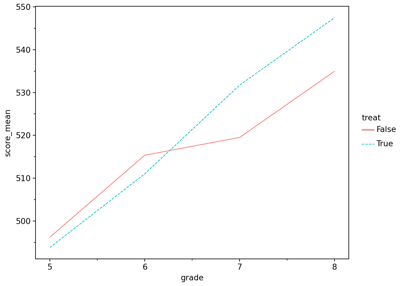
Figure 3.1 shows that the students who went to the camp had lower scores in grades 5 and 6 (i.e., before the camp), but stronger performance in grades 7 and 8. This provides prima facie evidence of a positive effect of the science camp on scores. In this context we are considering attendance at the science camp as a kind of “treatment” that some “patients” receive, hence treat.
While the ideal approach might be to randomly assign students to the camp and then compare scores after the camp, in this case, it appears that students with lower scores went to camp. Given our lack of contextual information, there is no obvious story for what we see in Figure 3.1 that is more plausible than (or at least as simple as) one that attributes a positive effect on test scores of going to the science camp.
A question that we might now have is: What is the best way to test for an effect of the science camp on test scores? One reasonable hypothesis is that the summer camp has a biggest effect on seventh-grade scores and that we might compare seventh-grade scores with sixth-grade scores to get the best estimate of the effect of camp on scores.
In the code below, we use .filter() to limit our analysis to data related to sixth and seventh grades. We then calculate mean scores for each value of ["post", "treat"]. We then use .pivot() to put score values for different levels of post in the same row so that we can calculate change.
test_summ = (
    camp_scores
    .filter(pl.col("grade").is_in([6, 7]))
    .group_by("post", "treat")
    .agg(pl.col("score").mean())
    .pivot(on="post", values="score")
    .rename({"true": "post", "false": "pre"})
    .with_columns(change=pl.col("post") - pl.col("pre"))
)
You may find it helpful in understanding method chains (or “pipelines”) such as this one to look at the intermediate output along the pipeline. For example, remove the assignment to test_summ and comment out the lines after the .agg() line and run that, you can see what is coming out at that point of the method chain:
# test_summ =
(
    camp_scores
    .filter(pl.col("grade").is_in([6, 7]))
    .group_by(["post", "treat"])
    .agg(pl.col("score").mean())
    # .pivot(on="post", index="treat", values="score")
    # .rename({"true": "post", "false": "pre"})
    # .with_columns(change=pl.col("post") - pl.col("pre"))
)
We strongly recommend that you use this approach liberally when working through this book (and when debugging your own pipelines).
We stored the results of our analysis in the data frame test_summ, which we show in Table 3.1.
test_summ.with_columns(pl.col(pl.Float64).round(3))| treat | pre | post | change |
|---|---|---|---|
| true | 511.016 | 531.729 | 20.713 |
| false | 515.354 | 519.515 | 4.161 |
We see in Table 3.1 that the mean score of the treated students (i.e., those who went to the summer camp) increased by 20.713, while the mean score of the control students increased by 4.161.
One approach is to view the outcome of the control students as the “but-for-treatment” outcome that the treated students would have seen had they not gone to summer camp. With this view, the effect of going to camp is the difference in the change in the scores between the two groups, or 16.552. This is the difference-in-differences estimator of the causal effect that we study more closely in Chapter 19.
We can also recover this estimator using the smf.ols() function. Polars provides a .pipe() method on DataFrame objects that allows functions to be inserted naturally into a method chain, playing a role similar to the pipe operator (|> or %>%) in R. The ols_fit() function that we defined above, is already “pipe-friendly”, as we put the data argument in the first position.
fm_dd = (
    camp_scores
    .filter(pl.col("grade").is_in([6, 7]))
    .pipe(ols_fit, formula="score ~ treat * post")
)
fm_dd.params
Intercept 515.353836
treat[T.True] -4.337714
post[T.True] 4.161014
treat[T.True]:post[T.True] 16.551796
dtype: float64Note that, as before, we did not need to specify the inclusion of the main effects of treat and post; smf.ols() automatically added those when we requested their interaction (treat * post). Also note that we did not need to convert the logical variables treat and post so that True is 1 and False is 0; in effect, smf.ols() also did this for us.
A natural question might be whether we could do better using all four years of data. There is no simple answer to this question unless we have a stronger view of the underlying causal model. One causal model might have it that students have variation in underlying talent, but that there is also variation in industriousness that affects how students improve over time. From the perspective of evaluating the effect of the camp, variation in industriousness is going to add noise to estimation that increases if we are comparing performance in fifth grade with that in eighth grade.
Another issue is that the effects of the summer camp might fade over time. As such, we might get a larger estimated effect if we focus on seventh-grade scores than if we focus on (or also include) eighth-grade scores. But from a policy perspective, we might care more about sustained performance improvement and actually prefer eighth-grade scores.
However, if we were willing to assume that, in fact, scores are a combination of underlying, time-invariant individual talent, the persistent effects (if any) of summer camp, and random noise, then we’d actually do better to include all observations.4
fm_dd_all = (
    camp_scores
    .pipe(ols_fit, formula="score ~ treat * post")
)

fm_dd_all.params
Intercept 505.791165
treat[T.True] -3.377287
post[T.True] 21.454769
treat[T.True]:post[T.True] 15.735784
dtype: float64Another possibility is that scores are a combination of underlying, time-invariant individual talent, the persistent effects (if any) of summer camp, and random noise and the grade in which the test is taken. For example, perhaps the test taken in seventh grade is similar to that taken in sixth grade but, with an extra year of schooling, students might be expected to do better in the higher grade assuming the scores are not scaled in any way within grades. (Recall that we just have this data set without details that would allow us to rule out such ideas, so the safest thing to do is to examine the data.)
The easiest way to include grade is as a linear trend, which means that grade is viewed as a number (e.g., 5 or 8):
fm_dd_trend = (
    camp_scores
    .pipe(ols_fit, formula="score ~ treat * post + grade")
)print(fm_dd_trend.params)Intercept 412.919547
treat[T.True] -3.377287
post[T.True] -12.316729
treat[T.True]:post[T.True] 15.735784
grade 16.885749
dtype: float64Note that we have exactly the same coefficients on treat and treat * post as we had before (-3.377 and 15.736, respectively). The easiest way to understand the estimated coefficients is to plug in some candidate \(X\) values to get the fitted values.
Suppose we have a student who went to summer camp. In grade 6, this student’s predicted score would be
\[ 412.9195 + -3.3773 + 6 \times 16.8857 = 510.8568 \]
In grade 7, this student’s predicted score would be
\[ 412.9195 + -3.3773 + 7 \times 16.8857 + 15.7358 = 543.4783 \]
An alternative approach that allows for the possibility that grade affects scores is to estimate a separate intercept for each level of grade. That is, we could have a different intercept for grade==6, a different intercept for grade==7, and so on.
Rather than adding dummy variables for grade to the model above, let’s run a simpler regression and use C() to tell the formula parser to treat grade as a categorical variable rather than as a numerical one. Categorical variables often have no meaningful numerical representation (e.g., “red” or “blue”, or “Australia” or “New Zealand”) or we may want to move away from a simple numerical representation (e.g., grade 7 may not be simply 7/6 times grade 6).5
fm_grade = (
    camp_scores
    .pipe(ols_fit, formula="score ~ C(grade)")
)
fm_grade.params
Intercept 495.020063
C(grade)[T.6] 18.164916
C(grade)[T.7] 30.601827
C(grade)[T.8] 46.208409
dtype: float64This model estimates fixed effects for each grade without other covariates. Table 3.2 provides the mean scores by grade for comparison.
| grade | score |
|---|---|
| 5 | 495.02 |
| 6 | 513.185 |
| 7 | 525.622 |
| 8 | 541.228 |
The idea of fixed effects is that there are time-invariant factors that have a constant effect on the outcome (hence fixed effects). In some settings, we would posit fixed effects at the level of the individual. Here we are positing fixed effects at the grade level. Working through the exercises should provide additional insights into what we are doing here. For more on fixed effects, see Cunningham (2021, pp. 391–392) and also Chapter 21.
Now, let’s estimate fixed effects for both grade and student (id). This will yield more fixed effects than we have students (we have 1000 students), so for reasons of space we suppress the coefficients for the fixed effects in the regression output, which is shown in Table 3.3.
Note
The helper ols_dropcollinear() provided by the era_pl package fits the same OLS model we would otherwise estimate with smf.ols(), but first removes regressors that are exact linear combinations of the others. This is needed here because a model with an intercept, grade fixed effects, student fixed effects, and treatment indicators will have collinear regressors. Later in the book we will often use packages such as pyfixest, which handle this kind of collinearity automatically by dropping redundant variables for us.
fm_id = (
    ols_dropcollinear(
        data=camp_scores,
        formula="score ~ treat * post + C(grade) + C(id)")
)

ETable(
    [fm_id],
    coef_fmt="b:.3f* \n (t:.3f)",
    signif_code=[0.01, 0.05, 0.10],
    model_stats=["N", "r2"],
    drop=["C\\(grade\\)", "C\\(id\\)"],
)
Model matrix is rank deficient.
Parameters were not estimable:
'C(grade)[T.7]', 'C(id)[T.29]'grade and id fixed effects
| y | |
|---|---|
| (1) | |
| coef | |
| treat=True | -5.148 (-1.476) |
| post=True | 22.734*** (84.240) |
| treat=True × post=True | 15.736*** (50.496) |
| Intercept | 486.404*** (197.044) |
| stats | |
| Observations | 4,000 |
| R2 | 0.949 |
| Significance levels: * p < 0.1, ** p < 0.05, *** p < 0.01. Format of coefficient cell: Coefficient (t-stats) | |
The fitted model stores the \(X\) matrix used in estimation as fm_id.model.exog. The size of this matrix is given by it shape attribute:
X = fm_id.model.exog
X.shape
(4000, 1004)We have 1004 columns because we have added so many fixed effects. This means that \((X^{\mathsf{T}}X)^{-1}\) is a 1004 \(\times\) 1004 matrix. As we add more years and students, this matrix could quickly become quite large and inverting it would be computationally expensive (even more so for some other operations that would need even larger matrices). To get a hint as to a less computationally taxing approach, let’s see what happens when we “demean” the variables in a particular way.
camp_scores_demean = (
    camp_scores
    .with_columns(
        pl.col("score") - pl.col("score").mean().over("id")
    )
    .with_columns(
        pl.col("score") - pl.col("score").mean().over("grade")
    )
)

fm_demean = (
    camp_scores_demean
    .pipe(ols_fit, "score ~ treat * post")
)
Notepandas
The expression pl.col("score").mean().over("id") is the Polars analogue of something like df.groupby("id")["score"].transform("mean") in pandas. The important point is that over("id") returns one value per original row rather than collapsing the data to one row per group.
Results from this analysis are shown in Table 3.4.
ETable(
    [fm_demean],
    coef_fmt="b:.3f* \n (t:.3f)",
    signif_code=[0.01, 0.05, 0.10],
    model_stats=["N", "r2"],
)| score | |
|---|---|
| (1) | |
| coef | |
| treat=True | -7.868*** (-41.237) |
| post=True | -7.868*** (-41.237) |
| treat=True × post=True | 15.736*** (58.318) |
| Intercept | 3.934*** (29.159) |
| stats | |
| Observations | 4,000 |
| R2 | 0.46 |
| Significance levels: * p < 0.1, ** p < 0.05, *** p < 0.01. Format of coefficient cell: Coefficient (t-stats) | |
The size of the \(X\) matrix is now 4000 \(\times\) 4. This means that \((X^{\mathsf{T}}X)^{-1}\) is now a much more manageable 4 \(\times\) 4 matrix. While we had to demean the data, this is a relatively fast operation.
3.2.3 Exercises
In using
.pivot()in creatingtest_summ, we did not supply a value for theindexargument. What value was implicitly used in the code creatingtest_summ?What is the relation between the means in Table 3.2 and the regression coefficients in
fm_grade?Why is there no estimated coefficient for
grade=5infm_grade?Now let’s return to our earlier regression specification, except this time we include fixed effects for
grade(see code below and output in Table 3.5). We now have two omitted grade indicators:grade=5andgrade=8. Why are we now losing two grade indicators, while above we lost just one? (Hint: Which variables can be expressed as linear combinations of thegradeindicators?)
fm_dd_fe = (
    camp_scores
    .pipe(ols_dropcollinear,
          formula="score ~  treat * post + C(grade)")
)
Model matrix is rank deficient.
Parameters were not estimable:
'C(grade)[T.8]'ETable(
[fm_dd_fe],
coef_fmt="b:.3f* \n (t:.3f)",
signif_code=[0.01, 0.05, 0.10],
model_stats=["N", "r2"],
)grade fixed effects
| y | |
|---|---|
| (1) | |
| coef | |
| treat=True | -3.377*** (-10.980) |
| post=True | 38.341*** (101.774) |
| grade=6 | 18.165*** (59.055) |
| grade=7 | -15.607*** (-50.738) |
| treat=True × post=True | 15.736*** (36.174) |
| Intercept | 496.709*** (1864.648) |
| stats | |
| Observations | 4,000 |
| R2 | 0.867 |
| Significance levels: * p < 0.1, ** p < 0.05, *** p < 0.01. Format of coefficient cell: Coefficient (t-stats) | |
In words, what are we doing to create
camp_scores_demean? Intuitively, why might this affect the need to use fixed effects?Can you relate the coefficients from the regression stored in
fm_demeanto the numbers in Table 3.6? of these estimated coefficients is meaningful? All of them? Some of them? None of them?
(
    camp_scores_demean
    .group_by(["grade", "treat"])
    .agg(pl.col("score").mean().alias("score"))
    .sort("grade", "treat")
    .style
    .fmt_number(columns="score", decimals=3)
)grade and treat
| grade | treat | score |
|---|---|---|
| 5 | false | 3.454 |
| 5 | true | −3.454 |
| 6 | false | 4.414 |
| 6 | true | −4.414 |
| 7 | false | −3.862 |
| 7 | true | 3.862 |
| 8 | false | −4.006 |
| 8 | true | 4.006 |
- The
feols()function from thepyfixestpackage offers a succinct syntax for adding fixed effects and uses computationally efficient algorithms (much like our demeaning approach above) in estimating these. What is the same in the results below and the two specifications we estimated above? What is different? Why might these differences exist? What is theI()function doing here? What happens if we omit it (i.e., just includepost * treat)?
fefm = pf.feols(
    fml="score ~ I(post * treat) | grade + id",
    data=camp_scores
)
fefm.coef()
Coefficient
I(post * treat) 15.735784
Name: Estimate, dtype: float643.3 Frisch-Waugh-Lovell theorem
The Frisch-Waugh-Lovell theorem states that the following two regressions yield identical regression results in terms of both the estimate \(\hat{\beta_2}\) and residuals.
\[ y = X_1 \beta_1 + X_2 \beta_2 + \epsilon \] and
\[ M_{X_1} y = M_{X_1} X_2 \beta_2 + \eta \]
where \(M_{X_1}\) is the “residual maker” for \(X_1\) or \(I - P_{X_1} = I - X_1({X_1^{\mathsf{T}}X_1})^{-1}X_1^{\mathsf{T}}\), \(y\) is a \(n \times 1\) vector, and \(X_1\) and \(X_2\) are \((n \times k_1)\) and \((n \times k_2)\) matrices.
In other words, we have two procedures that we can use to estimate \(\hat{\beta}_2\) in the regression equation above. First, we could simply regress \(y\) on \(X_1\) and \(X_2\) to obtain estimate \(\hat{\beta}_2\). Second, we could take the following more elaborate approach:
- Regress \(X_2\) on \(X_1\) (and a constant term) and store the residuals (\(\epsilon_{X_1}\)).
- Regress \(y\) on \(X_1\) (and a constant term) and store the residuals (\(\epsilon_{y}\)).
- Regress \(\epsilon_{y}\) on \(\epsilon_{X_1}\) (and a constant term) to obtain estimate \(\hat{\beta}_2\).
The Frisch-Waugh-Lovell theorem tells us that only the portion of \(X_2\) that is orthogonal to \(X_1\) affects the estimate \(\hat{\beta}_2\). Note that the partition of \(X\) into \([X_1 X_2]\) is quite arbitrary, which means that we also get the same estimate \(\hat{\beta_1}\) from the first regression equation above and from estimating
\[ M_{X_2} y = M_{X_2} X_1 \beta_1 + \upsilon \]
To verify the Frisch-Waugh-Lovell theorem using some actual data, we draw on the data set comp from the era_pl package and a regression specification we will see in Chapter 24.
comp = load_data("comp")As our baseline, we run the following linear regression and store it in fm.
base = (
    "big_n + size + lev + mtb + "
    "C(fyear) * (inv_at + I(d_sale - d_ar) + ppe)"
)

fm = ols_fit(comp, f"ta  ~ {base} + cfo")
Here the dependent variable is ta (total accruals), big_n is an indicator variable for having a Big \(N\) auditor (see Section 25.1), and the other variables are various controls that we discuss in more detail in Chapter 24, where we construct comp. We again use the I() function we saw above and interact C(fyear) with three different variables.
We then run two auxiliary regressions: one of ta on all regressors except cfo (we store this in fm_aux_ta) and one of cfo on all regressors except cfo (we store this in fm_aux_cfo).
fm_aux_ta  = ols_fit(comp, f"ta  ~ {base}")
fm_aux_cfo = ols_fit(comp, f"cfo ~ {base}")
We then take the residuals from each of these regressions and put them in a data frame under the names of the original variables (ta and cfo respectively).
aux_data = pl.DataFrame({
    "ta":  fm_aux_ta.resid,
    "cfo": fm_aux_cfo.resid
})
Finally, using the data in aux_data, we regress ta on cfo.
fm_aux = ols_fit(aux_data, "ta ~ cfo")The Frisch-Waugh-Lovell theorem tells us that the regression in fm_aux will produce exactly the same coefficient on cfo and the same residuals (and very similar standard errors) as the regression in fm, as can be seen in Table 3.7. Here we use ETable() from the maketables package to produce attractive regression output. We use drop = ["fyear", "ppe", "inv_at", "d_sale"] to focus on coefficients of greater interest.
ETable(
    [fm, fm_aux],
    model_heads=["Full model", "Auxiliary regression"],
    head_order="h",
    coef_fmt="b:.3f* \n (t:.3f)",
    signif_code=[0.01, 0.05, 0.10],
    model_stats=["N", "r2"],
    drop=["fyear", "ppe", "inv_at", "d_sale"],
)| Full model | Auxiliary regression | |
|---|---|---|
| (1) | (2) | |
| coef | ||
| big_n=True | 0.022* (1.956) |
|
| size | -0.000 (-0.182) |
|
| lev | -0.066*** (-5.210) |
|
| mtb | -0.000*** (-5.722) |
|
| cfo | 0.141*** (17.197) |
0.141*** (17.278) |
| Intercept | -0.061*** (-5.620) |
0.000 (0.000) |
| stats | ||
| Observations | 8,850 | 8,850 |
| R2 | 0.873 | 0.033 |
| Significance levels: * p < 0.1, ** p < 0.05, *** p < 0.01. Format of coefficient cell: Coefficient (t-stats) | ||
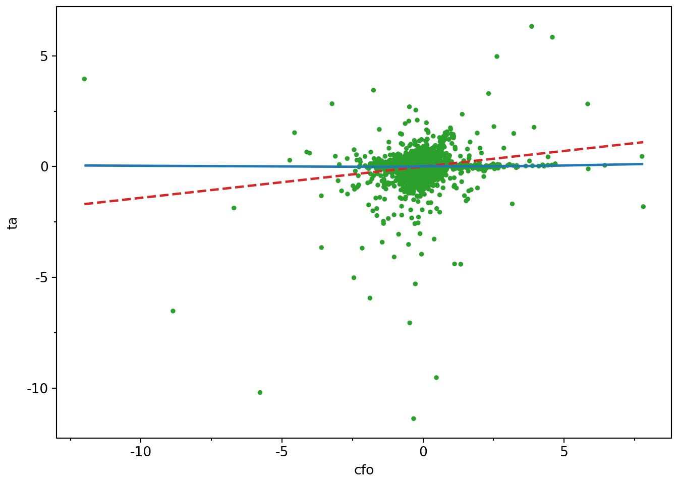
The Frisch-Waugh-Lovell theorem is an important result for applied researchers to understand, as it provides insights into how multivariate regression works. A side-benefit of the result is that it allows us to reduce the relation between two variables in a multivariate regression to a bivariate regression without altering that relation. For example, to understand the relation between cfo and ta embedded in the estimated model in fm, we can plot the data.
We produce two plots. The first–Figure 3.2—includes all data, along with a line of best fit and a smoothed curve of best fit. However, Figure 3.2 reveals extreme observations of the kind that we will study more closely in Chapter 24 (abnormal accruals more than 5 or less than 5 times lagged total assets!).
(
    aux_data
    .drop_nulls(subset=["cfo", "ta"])
    .ggplot(aes(x="cfo", y="ta"))
    .geom_point(size=1, color="tab:green")
    .geom_smooth(method="lm", se=False, linetype="--", color="tab:red")
    .geom_smooth(method="lowess", se=False, color="tab:blue")
)
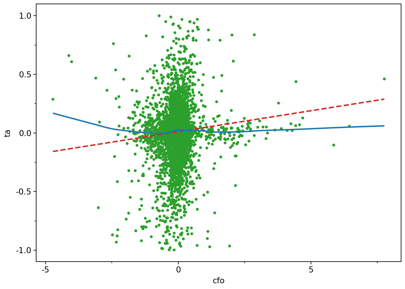
So we trim the values of ta at \(-1\) and \(+1\) and produce a second plot.6 In our second plot—Figure 3.3—there is no visually discernible relation between cfo and ta and the line of best fit is radically different from the curve. If nothing else, hopefully these plots raise questions about the merits of blindly accepting regression results with the messy data that we often encounter in practice.
(
    aux_data
    .drop_nulls(subset=["cfo", "ta"])
    .filter(pl.col("ta").abs() < 1)
    .ggplot(aes(x="cfo", y="ta"))
    .geom_point(size=1, color="tab:green")
    .geom_smooth(method="lm", se=False, linetype="--", color="tab:red")
    .geom_smooth(method="lowess", se=False, color="tab:blue")
)
3.3.1 Exercises
Verify the Frisch-Waugh-Lovell theorem using
big_nandlevin place ofcfoand produce plots like Figure 3.2 for each variable. Does the plot withbig_nas the independent variable seem less helpful?Above we said that the standard errors of the main regression and the auxiliary regression using the Frisch-Waugh-Lovell theorem should be “very similar”. Confirm that the standard errors are similar across the variants of
fmandfm_auxthat you calculated for the previous question. (Hint:fm_aux.bseandfm.bseprovide the estimated standard errors, whilefm_aux.df_residandfm.df_residprovide the residual degrees of freedom.) Can you guess what might explain any differences? (Hint: Compare the residual degrees of freedom and perhaps usenp.sqrt().)In words, what effect does converting
fyearinto a categorical variable and interacting it withinv_at,I(d_sale - d_ar), andppehave? (Hint: It may be helpful to visually inspect the more complete regression output produced withoutdrop=["fyear", "ppe", "inv_at", "d_sale"].)
3.4 Further reading
This chapter provides a bare minimum introduction to running regressions in Python plus some concepts that help develop intuition about what’s going on in OLS regression. Treatments that provide a similar emphasis on intuition, but go deeper into the details include Angrist and Pischke (2008) and Cunningham (2021). Any econometrics textbook will offer a more rigorous treatment of OLS and its properties.
An estimand is simply a fancy way of saying the thing we’re trying to estimate.↩︎
For a quick overview of some details of matrix algebra, see Appendix A.↩︎
The third argument to
smf.ols()issubset, which allows us to specify as condition that each observation needs to satisfy to be included in the regression.↩︎The idea here being that more data is better than less. This idea will show up again in later chapters.↩︎
An introduction to categorical data in Polars can be found at https://docs.pola.rs/user-guide/expressions/categorical-data-and-enums/.↩︎
That is, values less than \(-1\) are set to \(-1\) and values greater than \(+1\) are set to \(+1\). This is similar to winsorization, which we discuss in Chapter 24.↩︎