2  The basics of data analysis

This chapter aims to provide a brief, fast-paced introduction to both the fundamentals of data analysis in Python and basic statistics suitable even for someone with no knowledge of Python. Python is a programming language that also provides a software environment for performing statistical computing and creating graphics. Like a natural language, the best way to learn a computer language is to dive in and use it. Unlike a natural language, one can achieve a degree of fluency in a matter of hours. Also as a learner, you do not need to find a native speaker of Python willing to tolerate your bad grammar; you can practise Python without leaving your computer and get immediate feedback on your attempts.¹

As we assume very little here in terms of prior exposure to Python or statistics, some points in this chapter may seem a little tedious. But we expect these parts can be covered quickly. We highly recommend that you treat this chapter as a tutorial and work through the code that follows, either by typing or by copying and pasting into the Python console (this is what we mean by an “active reader” above). Once you have completed the steps described on the support page for this book, the code below should allow you to produce the output below on your own computer in this fashion. The idea of allowing the reader to produce all the output seen in this book by copying and pasting the code provided is a core commitment that we make to the reader.

Some parts of the code may seem a little mysterious or unclear. But just as one does not need to know all the details of the conditional tense in French to use Je voudrais un café, s’il vous plaît, you don’t need to follow every detail of the commands below to get a sense of what they mean and the results they produce (you receive a coffee). For one, most concepts covered below will be examined in more detail in later chapters.

In addition, you can easily find help for almost any task in Python’s documentation, other online sources, or in the many good books available on statistical computing (and we provide a guide to further reading at the end of this chapter).

We believe it is also helpful to note that the way even fluent speakers of computer languages work involves internet searches for things such as “how to reorder column charts using plotnine” or asking questions on StackOverflow or using large language models such as ChatGPT and Claude. To be honest, some parts of this book were written with such an approach. The path to data science fluency for many surely involves years of adapting code found on the internet to a problem at hand.

As such, our recommendation is to go with the flow, perhaps playing with the code to see the effect of changes or trying to figure out how to create a variant that seems interesting to you. To gain the most from this chapter, you should try your hand at the exercises at the end of chapter. As with the remainder of the book, these exercises often fill in gaps deliberately left in the text itself.

Tip

The Python code in this chapter assumes that you have set up your computer according to instructions on the book’s support page. The support page also includes Quarto templates for the code and exercises below.

2.1 An introduction to Python

2.1.1 Functions

Python contains a multitude of functions. For example, the math.exp() function computes the exponential function:

import math
math.exp(1)

2.718281828459045

After we have typed import math, we can access the documentation for math.exp() by typing help(math.exp) in Python (many ways of running Python, such as Jupyter also allow math.exp?). The documentation for math.exp() tells us that it takes one argument (x) and that it will “Return e raised to the power of x.”

In contrast, help(math.log) shows the form log(x, [base=math.e]). This tells us that math.log() takes up to two arguments. There is no default for the first argument x, but the second argument (base) has a default of math.e. So, if we supply on the first argument, math.log() returns the natural logarithm of the value supplied as the first argument.

math.log(8)

2.0794415416798357

To get base-10 logarithm, we can supply 10 as the second argument.

math.log(100, 10)

2.0

Creating new functions is quite straightforward, as can be seen in the following example.

def square(x):
    return x ** 2

We can now call our function like any other function:

square(2)

4

square(64)

4096

2.1.2 Operators

Like any programming language, Python has a full set of arithmetic operators, including +, *, and /. Here are some examples for you to try.

NoteInteractive output

When you run a block of code in an interactive Python environment, only the output of the last line is displayed. So, to see the full output of these examples, run each line one at a time.

2 + 2
4 * 3
5 / 2
16 ** 2

In Python, large numbers can be entered using _ to improve readability:

10_000_000

10000000

Another class of operators comprises the relational operators, such as >, >=, ==, and !=. As can be seen below, these operators yield either True or False.

6 > 4
6 < 4
6 == 4
6 != 4
6 == 3 + 3

Another class of operators in Python is the logical operators, including not, and, and or.

not (6 == 4)
not True
True and False
True or False

2.1.3 Variables

We can use the assignment operator = to store an object in a variable. For example, we can store 3 in the variable v as follows.

v = 3

We can then recover and manipulate this value later.

v

3

We can add 3 to v …

v + 3

6

… but doing so doesn’t change the value of v:

v

3

To add 4 to v and store that new value in v, we need to assign that new value to v.²

v = v + 4
v

7

2.1.4 Packages

When you start Python, a number of functions and types are immediately available, including the basic arithmetic operators and built-in functions such as len() and sum(). However, much of Python’s functionality is provided by packages.

Some packages are part of Python’s standard library (for example, math and statistics), while third-party packages must be installed separately. In setting up your computer using the instructions here, you will have installed a number of third-party packages, including numpy.³

Once a package has been installed, it can be imported into Python using the import statement. You may have noticed that we already used import math above.

2.2 Data fundamentals

2.2.1 Data types

Values stored in a computer will have well-defined data types, which determine how they behave and what operations can be applied to them. Different data types support different operations, use memory differently, and may lead us to make different analytical choices.

Some of the data types we encounter in this book are as follows.

• Numeric: values represent magnitudes or quantities, e.g. 123 or 3.14159265.
• Textual: values represent text, e.g., "Hello" or "000123".
• Logical: values represent whether a statement is true or false.
• Categorical: values indicate membership in a group or class.
• Temporal: values locate events in time or to represent spans of time.

These categories are partly conceptual. For example, the firm identifier gvkey that we see later in this chapter has six digits (e.g., 024512), and that could be stored either as a numeric type (24512) or as a textual type ("024512"). In this case, there is no value in treating it as numeric data in an analytical sense. For example, adding two gvkey firm identifiers or taking their average is not meaningful. Similarly, the four-digit code representing the industry in which a firm operates might be stored as an integer or as text, but conceptually it is categorical.

2.2.1.1 Numeric types

Even within numeric data, we often distinguish among multiple types.

• Integers: whole numbers such as counts, ranks, or identifiers that are genuinely whole-valued.
• Floating-point numbers: approximate representations of real numbers such as returns, ratios, and regression coefficients.
• Decimal or fixed-point numbers: numbers with a fixed number of digits after the decimal point, often used for currency or other values where exact decimal representation matters.

The distinction between integers and floating-point numbers matters because the set of sensible operations differs. If a variable counts the number of directors on a company’s board, an integer representation means that values such as 7.5 are impossible. Floating-point numbers are more flexible for continuous quantities, but they are usually only approximations. As such, values such as 0.1 may not be represented exactly in binary floating-point arithmetic, though such issues are not material for most calculations.

Decimal types are designed for cases where exact decimal representation is important. The standard Python decimal library provides the Decimal for such cases.⁴

2.2.1.2 Textual and logical types

Examples of textual data include company names, tickers, addresses, and free-form descriptions. A postal or ZIP code is a familiar example of data that looks numerical, but is better thought of as text where the characters happen to be digits.

A logical data type—sometimes called Boolean data—records whether some condition holds. In Python terms, think True or False. Examples include indicators for whether a firm paid a dividend, whether an observation passes a filter, or whether a filing is late. Logical values support operations such as filtering, combining conditions, and counting how often a condition is true.

2.2.1.3 Categorical types

Categorical data indicate which class or group an observation belongs to. Examples include exchange codes, industry classifications, and treatment or control labels. The important feature is that the values identify categories rather than magnitudes.

This distinction matters because the numerical labels attached to categories are usually arbitrary. If we code firms by industry as 1, 2, and 3, it does not follow that industry 3 is “larger” than industry 1 or that the difference between 3 and 2 is meaningful. Treating categorical data as if they were ordinary numbers can therefore produce nonsensical summaries or models.

2.2.1.4 Temporal types

Temporal data deserve separate treatment because time has structure that ordinary numbers do not. We will encounter several kinds of temporal values:

• Instants: points in time such as a date, a clock time, or a timestamp.
• Durations: elapsed amounts of time such as 30 days or 12 months.
• Periods: spans or intervals such as fiscal year 2024 or the quarter ending on March 31, 2024.

These distinctions matter because different operations make sense for different temporal objects. Subtracting one date from another yields a duration. Adding a duration to a date yields another date. By contrast, adding two dates together has no clear interpretation.

Python names some of its basic built-in types in straightforward ways. For example, int, float, str, and bool correspond to integers, floating-point numbers, text strings, and logical values, respectively. We can use the type() function to determine the type of a value. Here are some examples for you to try:

type(1)
type(3.1415) 
type("hello")
type(True)

2.2.2 Data structures

In doing data analysis, we rarely deal with single items of any of the types above. We will more often deal with collections of data items organized into some kind of data structure, whether provided by Python itself or by a third-party package.

2.2.2.1 Lists

One key data structure in Python is the list, which is an ordered collection of elements. We can create a list in Python using square brackets []:

l = [True, 1, 2.1, "frog"]

We access elements of a list using square brackets [] together with an index. Again Python uses zero-based indexing, so the first element is accessed with 0.

l[0]

True

l[3]

'frog'

List elements need not be of the same type. The first element of the list l is of Boolean type (bool) and the fourth element is a string (str).

type(l[0])

bool

type(l[3])

str

In fact, the elements of a list can be lists or other data structures themselves.

Note that extracting a single element of a list (e.g., l[0]) returns the element itself, not a one-element list. To extract a part of a list as a list, we can use a slice. In its most basic form, a slice includes start and stop and is usually written start:stop. For reasons related to Python’s use of zero-based indexing, a slice returns the elements with index i such that start <= i < stop. So, for example, l[1:3] returns the elements with indices 1 and 2.

We can omit start or stop. For example, l[start:] returns the elements with index i such that start <= i. And l[:stop] returns the elements with index i such that i < stop. Here are some examples to try:⁵

l2 = [1, 2, 3, 4, 5, 6, 7, 8]
l2[1:4]
l2[:4]
l2[4:]
l2[6:7]
l2[::2]

As with many things in Python, slices can be used in other contexts, such as strings. Here are some examples to try:

a_string = "I adore data analysis!"
a_string[0:4]
a_string[4]
a_string[::2]

For more on lists and slices, a good source is the official Python tutorial.

2.2.2.2 Dictionaries

Another fundamental Python data structure is the dictionary. A dictionary can be created using curly braces {}. For example, here we create three small dictionaries each with data about a single person:

anne = {"name": "Anne", "weight": 51}
bertha = {"name": "Bertha", "weight": 55, "height": 164}
charlie = {"name": "Charlie", "height": 184}

We can look up a value in a dictionary using the appropriate key:

anne["name"]

'Anne'

bertha["height"]

164

If we try anne["height"], we will get an error (try it for yourself). To avoid triggering a KeyError, we can use the .get() method.

anne_wgt = anne.get("height")
print(anne_wgt)

None

NoteKeys, not positions

Unlike lists, dictionaries are not designed to be accessed by position. Instead, dictionaries are designed to store items (i.e., key-value pairs), and we retrieve values using the relevant key.

In modern Python, dictionaries do preserve the order in which items were added. But that does not change the basic idea: when working with dictionaries, we normally access items by key, not by numeric position.

Instead of an error, we get the special Python value of None.

NoteMethods

A method is a special kind of function that attaches to an object. Different kinds of objects will have different methods according to what makes sense for that object. As anne is a dictionary (one kind of object), it comes with special functions that it can apply to itself.

In a way, you can think of it as equivalent to having a function get() that takes a dictionary as its first argument and the key as the second argument (i.e., get(anne, "height")). Using methods instead of functions allows objects in Python to carefully implement functions in ways that make the most sense for each kind of object. As with most idiomatic Python, the code in this book uses methods much more than it does functions.

To get more information about dictionaries, you can consult the Python documentation.

help(dict)

2.2.2.3 Arrays

Another fundamental data structure is the array. Arrays can be understood as a bit like lists, but with the constraint that each element of an array has to be of the same data type as all the other elements. While this sounds like a limitation, it’s actually a critical element of making operations on arrays fast enough (often extremely fast) to be a fundamental building block of the numerical analysis central to working with data.

While the Python standard-library array module provides array.array(...), this structure does not provide all the things that one wants from an array for data analysis. Instead, the de facto standard array structure used in data analysis is the ndarray provided by the third-party library NumPy (short for Numerical Python). It is conventional to import the NumPy library like this:

import numpy as np

This means we can refer to functions provided by NumPy using the abbreviated form np. One way to construct an ndarray uses np.array():

x = np.array([0, 1, 4, 9, 16, 25])
x

array([ 0,  1,  4,  9, 16, 25])

Because the ndarray is the de facto array in Python data science, we will just call them “arrays” henceforth. As you might expect, an array comes with a number of methods for the things you typically want to do with arrays. A compact reference to NumPy array functions, methods, and attributes used in this book is provided in Appendix Appendix B. Here are a few to try:

x.sum()
x.mean()
x.max()
x.min()

Arrays also have attributes, such as size or dtype

x.size

6

Each array has a single underlying data type (dtype).

x.dtype

dtype('int64')

NotePython

By now, you are probably starting to notice that many things in Python are objects. We have already learnt that an object comes with methods. Objects can also have attributes, which are like variables stored inside an object. We can access an attribute using the name of an object followed by a dot (.) followed by the attribute.

Scalar addition and multiplication of single-dimensional arrays work as you might if you think of them as vectors in linear algebra.⁶ That is, adding a scalar (a real number) to a vector adds that scalar to each element; multiplying a vector by a scalar multiplies each element by that scalar. Adding or multiplying two vectors means adding or multiplying each element (i.e., elementwise operations):

x * 2.5

array([ 0. ,  2.5, 10. , 22.5, 40. , 62.5])

x + 3

array([ 3,  4,  7, 12, 19, 28])

w = np.array([1, 2, 3, 4, 5, 6])
x + w

array([ 1,  3,  7, 13, 21, 31])

x * w

array([  0,   2,  12,  36,  80, 150])

When we attempt to mix values of different data types in a single array, NumPy converts them, when possible, to a type that can accommodate all values. So, a logical value can be interpreted as an integer (1 for True and 0 for False), an integer can be represented as a floating-point value, and a floating-point value (e.g., 3.1) can be thought of as a string ("3.1").

The following code demonstrates this: going from one line to the next, we add an element of a different type and the automatic conversion of the previous elements is evident from the output.

np.array([True, 2, 3.1])

array([1. , 2. , 3.1])

Here are some more examples to try:

np.array([True])
np.array([True, 2])
np.array([True, 2, 3.1, "frog"])

We can inspect the data type using the dtype attribute.

np.array([True, 2, 3.1]).dtype

dtype('float64')

Here are some more examples to try:

np.array([True]).dtype
np.array([True, 2]).dtype
np.array([True, 2, 3.1, "frog"]).dtype

A similar conversion can happen when we apply functions or methods to arrays. For example, summing a array of integers behaves as we would expect (here np.arange(1, 11) gives us the numbers from 1 to 10).

np.arange(1, 11).sum()

np.int64(55)

When sum() (or np.sum()) is applied to a Boolean array, True is treated like 1 and False is treated like 0:

v = np.array([True, True, False, False, False])

v.sum()

np.int64(2)

v.dtype

dtype('bool')

v.sum().dtype

dtype('int64')

Like lists, arrays use zero-based indexing and arrays elements can be accessed using []. So the first element is v[0] and the fourth is v[3].

v[0]

np.True_

v[3]  

np.False_

We have barely scratched the surface of the NumPy library here. Appendix B provides a useful reference for the functions and methods we used in this book. For further reading, the official NumPy documentation includes both NumPy: the absolute basics for beginners and the more extensive NumPy quickstart. Jake VanderPlas’s online Python Data Science Handbook also contains an excellent introduction to NumPy and several accessible follow-up sections on array operations.

2.3 Data frames

The final data structure we consider here is the data frame. Data frames are table-like (or spreadsheet-like) data structures in which each column represents a variable and each row represents an observation. Unlike arrays, the columns of a data frame may have different data types.

While standard Python does not include a data frame library, there are several third-party data frame libraries used for data analysis in Python. By far the most established data frame library is pandas, which has been the de facto standard data frame library in Python for more than a decade. Its broad adoption means that much existing Python code, documentation, and discussion of data analysis assumes some familiarity with pandas.

In recent years, other data frame libraries have emerged to address perceived limitations of pandas or to support special use cases. For example, PySpark provides a data frame interface designed for distributed computing across clusters, making it useful for very large data sets. Ibis offers a higher-level interface for working with data stored in databases. Recently Polars has attracted attention for its speed, efficiency, and expressive syntax.

In this book, we focus on Polars because its syntax makes data-manipulation code relatively easy to read while also scaling well to larger data sets.

2.3.1 Working with data frames

When working with data frames, it is helpful to think in terms of the verbs that represent the kinds of operations we want to perform on our data frames. Here are the most common things we want to do with data frames:

• filter rows based on their values
• arrange or reorder rows
• select columns
• mutate or create new variables from existing ones
• summarize many values into a smaller set of summary statistics

As you might expect by now, a Python data frame library will implement the operations as methods.

We first import the Polars package using its standard abbreviation (pl).

import polars as pl

To explore the methods provided by Polars, we will start with the aus_bank_funds data set provided with the era_pl Python package, which was created to support this book.

from era_pl import load_data

NotePython

Python offers different forms of the import statement. The command import polars as pl imports the polars package and assigns it the short alias pl, a conventional abbreviation that makes later code easier to read. By contrast, from era_pl import load_data imports only the load_data() function from the era_pl package, allowing us to call load_data() in later code without prefixing it with the package name.

We next load some data into a Polars DataFrame and assign it to aus_bank_funds.

aus_bank_funds = load_data("aus_bank_funds")

We can type aus_bank_funds at the Python console, Polars shows a compact summary of its contents:

aus_bank_funds

shape: (283, 7)

gvkey	datadate	at	ceq	ib	xi	do
str	date	f64	f64	f64	f64	f64
"024512"	1987-06-30	43886.853	2469.044	197.568	0.0	0.0
"024512"	1988-06-30	50445.3	2692.8	359.1	0.0	0.0
"024512"	1989-06-30	60649.6	3055.0	476.2	0.0	0.0
"024512"	1990-06-30	67030.1	3887.5	524.3	0.0	0.0
"024512"	1991-06-30	89292.1	4353.3	883.3	0.0	0.0
…	…	…	…	…	…	…
"200571"	1992-06-30	5263.165	331.272	6.082	0.0	0.0
"200571"	1993-06-30	6264.026	356.763	53.791	0.0	0.0
"200571"	1994-06-30	7330.519	503.752	62.989	0.0	0.0
"200571"	1995-06-30	8206.235	558.673	78.92	0.0	0.0
"200571"	1996-06-30	9197.325	617.021	91.209	0.0	0.0

The aus_bank_funds data frame contains selected annual financial statement data for Australian banks. The line shape: (283, 7) tells us that aus_bank_funds has 283 rows and 7 columns.⁷

The next two lines list the column names (gvkey, datadate, at, and so on) and their data types (str for text, date for dates, and f64 for numeric values stored as 64-bit floating-point numbers). The rows shown above are only a preview of the data rather than the entire data set, and Polars indicates the presence of additional rows using .... The definitions of the variables in aus_bank_funds are given in Table 2.1. Investors often refer to the kind of information provided in aus_bank_funds as fundamental data, as it relates to the operating performance of the business used in fundamental valuation analysis. Here the fundamental items come from the income statements and balance sheets for the respective firms and years and are presented in millions of Australian dollars.

Table 2.1: Variable definitions for aus_bank_funds

Variable	Meaning
gvkey	Firm identifier
datadate	Fiscal year-end date
at	Total assets
ceq	Common equity
ib	Income before extraordinary items
xi	Extraordinary items
do	Discontinued operations

By default, Polars will print out 10 rows. To save on space in this session, we can choose a different value using pl.Config:

pl.Config.set_tbl_rows(6)

polars.config.Config

2.3.2 Filtering rows with .filter()

The Polars DataFrame method .filter() accepts Boolean expressions (i.e., those that evaluate to True or False). To focus on fundamental data for periods ending after 1 January 2020, we can use the following statement:

aus_bank_funds.filter(pl.col("datadate") > pl.date(2020, 1, 1))

shape: (24, 7)

gvkey	datadate	at	ceq	ib	xi	do
str	date	f64	f64	f64	f64	f64
"024512"	2020-06-30	1.01406e6	72008.0	7459.0	2175.0	2175.0
"024512"	2021-06-30	1.091962e6	78713.0	8843.0	1338.0	1338.0
"024512"	2022-06-30	1.21526e6	72833.0	9673.0	1098.0	1098.0
…	…	…	…	…	…	…
"312769"	2022-06-30	1435.284	190.376	-12.391	72.178	72.178
"015362"	2020-09-30	911946.0	68023.0	2290.0	null	null
"015362"	2021-09-30	935877.0	72035.0	5458.0	null	null

There are a few things to note here. First, to make it clear that we are referring to a column of a data frame in certain contexts, we need to use the function pl.col(). Second, Polars is quite strict about data types and thus we need to use pl.date() to refer to dates rather than, say, using a string like "2020-01-01".⁸

2.3.3 Arranging rows with .sort()

We can sort rows by telling the Polars DataFrame method .sort() the columns we want to sort on. Because the inputs to .sort() are always column names, we don’t need to use pl.col() in this context.

aus_bank_funds.sort("datadate")

shape: (283, 7)

gvkey	datadate	at	ceq	ib	xi	do
str	date	f64	f64	f64	f64	f64
"024512"	1987-06-30	43886.853	2469.044	197.568	0.0	0.0
"015889"	1987-09-30	65310.023	3138.64	385.153	11.588	40.323
"014802"	1987-09-30	46971.5	2847.7	321.7	0.0	0.0
…	…	…	…	…	…	…
"312769"	2022-06-30	1435.284	190.376	-12.391	72.178	72.178
"200575"	2022-08-31	99930.0	6685.0	426.0	null	null
"015889"	2022-09-30	1.085729e6	65907.0	7138.0	-19.0	-19.0

We can supply multiple columns to .sort() and Polars will sort by the first column, then by the second column, and so on.

aus_bank_funds.sort("gvkey", "datadate")

shape: (283, 7)

gvkey	datadate	at	ceq	ib	xi	do
str	date	f64	f64	f64	f64	f64
"014802"	1987-09-30	46971.5	2847.7	321.7	0.0	0.0
"014802"	1988-09-30	63673.5	4096.6	569.4	0.0	0.0
"014802"	1989-09-30	76143.1	5555.3	791.6	0.0	0.0
…	…	…	…	…	…	…
"350949"	2020-06-30	2441.651	543.018	-50.844	null	null
"350949"	2021-06-30	7176.198	1075.892	28.808	null	null
"350949"	2022-06-30	9414.6	1404.6	-7.7	null	null

The default sort order is ascending, but we can supply descending=True to reverse that. If we are sorting on multiple columns, we can supply a list to Boolean values to indicate whether we want the sorting for column to be ascending or descending:

aus_bank_funds.sort("gvkey", "datadate", 
                    descending=[False, True])

shape: (283, 7)

gvkey	datadate	at	ceq	ib	xi	do
str	date	f64	f64	f64	f64	f64
"014802"	2021-09-30	925968.0	62779.0	6468.0	-104.0	-104.0
"014802"	2020-09-30	866565.0	61292.0	3494.0	-935.0	-935.0
"014802"	2019-09-30	847124.0	55596.0	5087.0	-289.0	-289.0
…	…	…	…	…	…	…
"350949"	2021-06-30	7176.198	1075.892	28.808	null	null
"350949"	2020-06-30	2441.651	543.018	-50.844	null	null
"350949"	2019-06-30	392.698	197.463	-27.966	null	null

NotePositional and keyword arguments

Python functions and methods can receive arguments either as positional arguments or as keyword arguments. With positional arguments, Python matches inputs according to their order. With keyword arguments, Python matches inputs using parameter names.

In .sort() above, the first two arguments are supplied as positional arguments, while the last one is supplied using the keyword descending.

In the code below, everything before end is positional and only end is a keyword argument.

print("This", "is", "a", "sentence", end=".\n")

This is a sentence.

With positional arguments, meaning depends on order. With keyword arguments, meaning depends on parameter names.

Python also lets us unpack values into a function call. Prefixing a list with * unpacks its elements as positional arguments, and prefixing a dictionary with ** unpacks its items as keyword arguments. We can see this in action below:

words = ["This", "is", "a", "sentence"]
keyword_args = {"end": ".\n"}

print(*words, **keyword_args)

This is a sentence.

In an ordinary function call, positional arguments need to be written before keyword arguments.

2.3.4 Selecting columns with .select()

If we were only interested in ib and ceq for period (datadate) for each company (gvkey), we can use the Polars DataFrame method .select() to get just those columns. Again, because it is obvious that we are referring to columns, we don’t need to use pl.col() in this context.

aus_bank_funds.select("gvkey", "datadate", "ib", "ceq")

shape: (283, 4)

gvkey	datadate	ib	ceq
str	date	f64	f64
"024512"	1987-06-30	197.568	2469.044
"024512"	1988-06-30	359.1	2692.8
"024512"	1989-06-30	476.2	3055.0
…	…	…	…
"200571"	1994-06-30	62.989	503.752
"200571"	1995-06-30	78.92	558.673
"200571"	1996-06-30	91.209	617.021

2.3.5 Creating new variables

We can actually use .select() to create new variables.

A bank’s income is likely to be an increasing function of shareholders’ equity. Banks’ return on assets generally come in the form of interest on loans to businesses and consumers, so more assets generally means more income. Assets equal liabilities plus shareholders’ equity and bank regulators normally insist on limits on the amount of assets based on the amount of shareholders’ equity.

For these reasons, a common measure of bank performance is return on equity, which we can calculate as:⁹

\[roe = \frac{ib}{ceq}\]

If we wanted a crude measure of return on equity (ROE) calculated as ib divided by ceq, we could simply do the following:

aus_bank_funds.select("gvkey", "datadate", "ib", "ceq",
                      roe = pl.col("ib") / pl.col("ceq"))

shape: (283, 5)

gvkey	datadate	ib	ceq	roe
str	date	f64	f64	f64
"024512"	1987-06-30	197.568	2469.044	0.080018
"024512"	1988-06-30	359.1	2692.8	0.133356
"024512"	1989-06-30	476.2	3055.0	0.155876
…	…	…	…	…
"200571"	1994-06-30	62.989	503.752	0.12504
"200571"	1995-06-30	78.92	558.673	0.141263
"200571"	1996-06-30	91.209	617.021	0.147822

Here we have expanded our select statement to include an additional column (roe) calculated using ib and ceq. In this context, we need to use pl.col() to make it clear that the inputs to the calculation are columns.

In some situations, we might want to simply add new columns to the existing columns. One approach would be to use the function pl.all() to select all existing columns and then supply calculations for any additional columns.

aus_bank_funds.select(pl.all(),
                      roe = pl.col("ib") / pl.col("ceq"))

shape: (283, 8)

gvkey	datadate	at	ceq	ib	xi	do	roe
str	date	f64	f64	f64	f64	f64	f64
"024512"	1987-06-30	43886.853	2469.044	197.568	0.0	0.0	0.080018
"024512"	1988-06-30	50445.3	2692.8	359.1	0.0	0.0	0.133356
"024512"	1989-06-30	60649.6	3055.0	476.2	0.0	0.0	0.155876
…	…	…	…	…	…	…	…
"200571"	1994-06-30	7330.519	503.752	62.989	0.0	0.0	0.12504
"200571"	1995-06-30	8206.235	558.673	78.92	0.0	0.0	0.141263
"200571"	1996-06-30	9197.325	617.021	91.209	0.0	0.0	0.147822

Another approach, which we will use more often in this book, uses .with_columns(...), which is a shortcut for select(pl.all(), ...). Here we use .with_columns() to calculate ROE and save the result to a new data frame aus_bank_roes.

aus_bank_roes = (
    aus_bank_funds
    .with_columns((pl.col("ib") / pl.col("ceq")).alias("roe"))
)

NotePolars

Note that we can use either positional or keyword arguments with .select() and .with_columns(). When we said roe = with .select(), we had roe as a keyword that is used by Polars to name the resulting column. But in the code just above, we did only supplied a single positional argument to .with_columns() and used .alias("roe") to ensure that the resulting column was named roe.

In idiomatic Polars usage, both approaches will be used according to what produces the most concise and readable code to produce the desired result.

As always, any positional arguments need to come before any keyword arguments.

Notepandas

Readers coming from pandas may be accustomed to using similar syntax for both methods and columns. For example, filtering can be done using syntax such as df[df["x"] > 0] and selecting columns using code like df[["a", "b"]]. This style can make row and column operations in pandas feel like variations on the same idea. Polars maintains a much stronger distinction between operations on rows such as .filter() and operations on columns such as .select() or .with_columns().

2.3.6 Summarizing using .group_by() and .agg()

Suppose we were interested in the average ROE for each firm in our sample. To do this, we group by the firm identifier using .group_by("gvkey") and then aggregate the data into a single value using the .mean() method.

(
    aus_bank_funds
    .with_columns(roe = pl.col("ib") / pl.col("ceq"))
    .group_by("gvkey")
    .agg(avg_roe = pl.col("roe").mean())
    .sort("avg_roe")
)

shape: (14, 2)

gvkey	avg_roe
str	f64
"350949"	-0.053491
"312769"	0.026814
"200695"	0.083285
…	…
"200051"	0.143385
"024512"	0.148018
"212631"	0.149412

NotePolars

Because the Polars methods we are using here are DataFrame methods that return a DataFrame, we can chain them together to create so-called method chains. This creates something resembling a pipeline where data flows from one operation to the next, as can be seen in the code above. Note that we need to place the whole pipeline in parentheses (i.e., ( and )) so that Python knows that everything inside is to be evaluated together. (An alternative would be to put everything on one line, but that would be more difficult to read.)

One benefit of method chains is that they avoid the need to create intermediate variables that immediately get overwritten, creating code that can be more difficult to understand.

We will return to our calculation of ROE later on. The era_pl package includes two additional data sets related to Australian banks. The first is aus_banks, which contains firm identifiers, tickers, and names of banks. The definitions of the variables in aus_banks are given in Table 2.2.

Table 2.2: Variable definitions for aus_banks

Variable	Meaning
gvkey	Firm identifier
ticker	Stock ticker
co_name	Company name

aus_banks = load_data("aus_banks")
aus_banks

shape: (10, 3)

gvkey	ticker	co_name
str	str	str
"014802"	"NAB"	"National Australia Bank Ltd"
"015362"	"WBC"	"Westpac Banking Corp"
"015889"	"ANZ"	"ANZ Bank New Zealand Limited"
…	…	…
"203646"	"SGB"	"St. George Bank Ltd"
"212631"	"BWA"	"Bank Of Western Australia"
"312769"	"BBC"	"BNK Banking Corp Ltd"

The second additional data frame is aus_bank_rets, which contains monthly data on stock returns and market capitalization for Australian banks. The definitions of the variables in aus_bank_rets are given in Table 2.3. As in many financial data sets, a value of 0.148 in ret indicates a 14.8% monthly return.

Table 2.3: Variable definitions for aus_bank_rets

Variable	Meaning
gvkey	Firm identifier
datadate	Observation date
ret	Monthly stock return
mkt_cap	Market capitalization

aus_bank_rets = load_data("aus_bank_rets")
aus_bank_rets

shape: (3_047, 4)

gvkey	datadate	ret	mkt_cap
str	date	f64	f64
"014802"	1985-12-31	null	1527.38458
"014802"	1986-01-31	0.083333	1654.666628
"014802"	1986-02-28	0.097713	1828.345559
…	…	…	…
"312769"	2022-08-31	-0.015625	74.782725
"312769"	2022-09-30	-0.111111	66.473533
"312769"	2022-10-31	0.116071	74.199628

One thing to note about the three data frames is that, while each covers the same Australian banks, they differ significantly in their number of rows, which reflects how many times each bank appears in each data set. In aus_banks, each bank appears only once. In contrast, aus_bank_funds contains multiple years of data per bank, and aus_bank_rets contains multiple monthly observations per bank.

2.4 Combining data frames

Suppose we are interested in making a plot of the market capitalization of Australian banks using the latest available data in aus_bank_rets.

We can apply the .max() method to the datadate column of aus_bank_rets to determine what we mean by “the latest available data”.

latest_date = aus_bank_rets.select("datadate").max().item()
latest_date

datetime.date(2022, 10, 31)

This suggests that we want to take a subset of the aus_bank_rets data having datadate equal to this value (assuming that the latest available date is the same for all banks in the table). But rather than working with latest_date, we can incorporate it into our .filter() directly:

latest_mkt_cap = (
    aus_bank_rets
    .filter(pl.col("datadate") == pl.col("datadate").max())
    .select("gvkey", "datadate", "mkt_cap")
    .sort("mkt_cap", descending=True)
    .rename({"mkt_cap": "Market capitalization"})
)

Notepandas

Users of pandas might be accustomed to viewing a DataFrame as a collection of Series objects (i.e., the individual columns) and doing a lot work using Series objects directly. For example, a pandas user would likely write latest_date = aus_bank_rets["datadate"].max(). While this is valid Polars code, for reasons that should become clearer when we start working with larger data sets, we generally avoid working with Series when working with Polars data frames. Additionally, method chains in Polars often facilitate the omission of intermediate assignments like latest_date = ....

Once we have the data, making a plot is easy. Here we use the plotnine_polars package to create Figure 2.1. (We discuss plotnine_polars in more detail in Section 2.7.1.)

from plotnine_polars import aes

(
    latest_mkt_cap
    .ggplot(aes(x="gvkey", y="Market capitalization"))
    .geom_col()
)

Figure 2.1: Market capitalization of Australian banks (initial version)

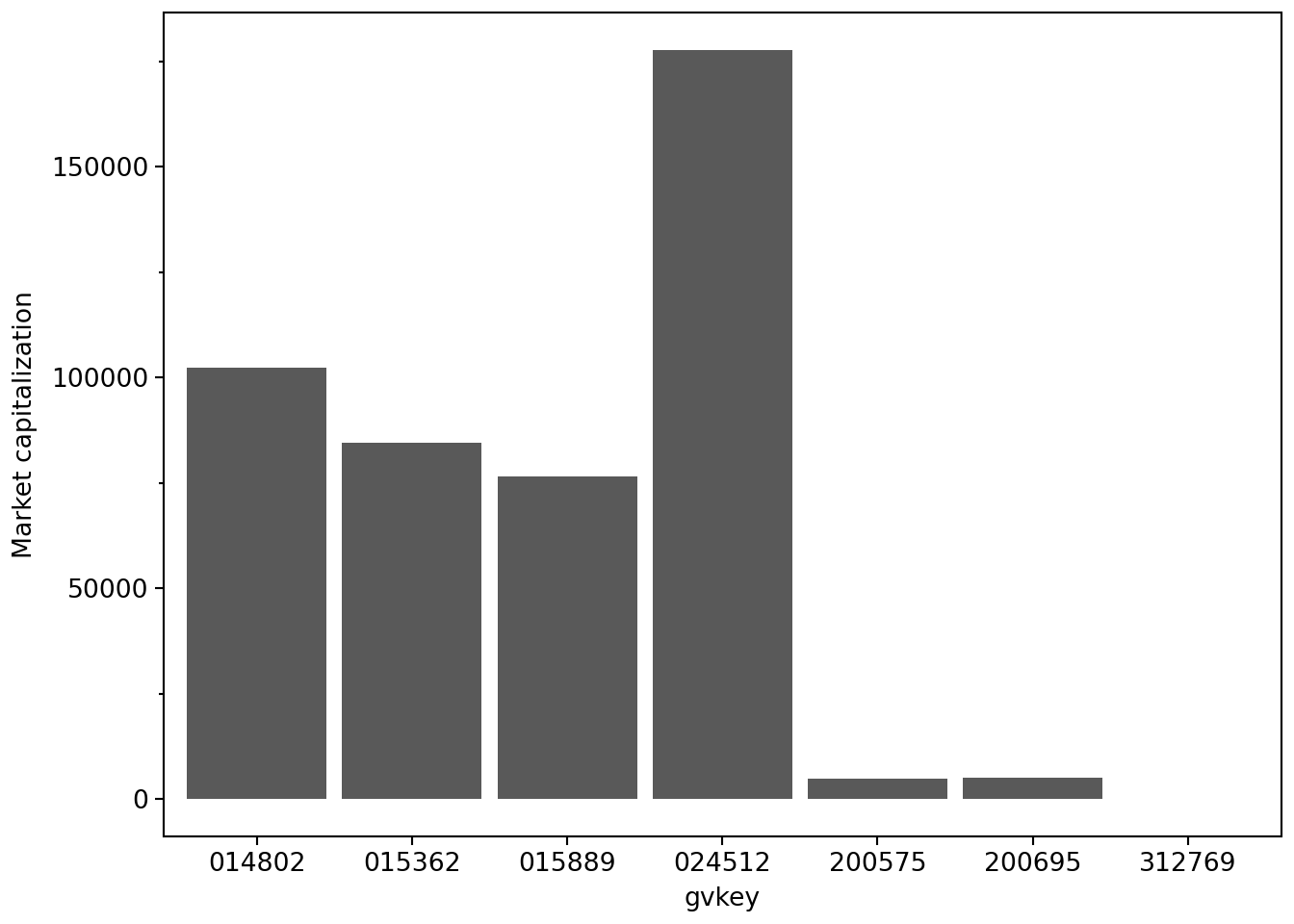
The immediate issue we see in Figure 2.1 is that we have no idea who these banks are. All we have in aus_bank_rets is the gvkey values, which no normal human can understand. A better plot would have the names of the banks, but these are in the aus_banks data frame, which has names and tickers but lacks data on market capitalization. We therefore need to combine information from these two tables to make the plot we want.

2.4.1 Combining tables using .join()

In Polars, we merge or join tables using the .join() method. Below we apply the .join() method to aus_banks and the first argument to .join() is the other table we are merging with (aus_bank_rets in our case). We specify the variables on which the join will be performed using the on argument and finally specify the type of join using how.

aus_banks_merged = (
    aus_banks
    .join(aus_bank_rets, on="gvkey", how="inner")
)

aus_banks_merged

shape: (3_047, 6)

gvkey	ticker	co_name	datadate	ret	mkt_cap
str	str	str	date	f64	f64
"014802"	"NAB"	"National Australia Bank Ltd"	1985-12-31	null	1527.38458
"014802"	"NAB"	"National Australia Bank Ltd"	1986-01-31	0.083333	1654.666628
"014802"	"NAB"	"National Australia Bank Ltd"	1986-02-28	0.097713	1828.345559
…	…	…	…	…	…
"312769"	"BBC"	"BNK Banking Corp Ltd"	2022-08-31	-0.015625	74.782725
"312769"	"BBC"	"BNK Banking Corp Ltd"	2022-09-30	-0.111111	66.473533
"312769"	"BBC"	"BNK Banking Corp Ltd"	2022-10-31	0.116071	74.199628

Here we have gvkey on both tables and can simply use on="gvkey". In some cases the common variables we wish to use to join the tables will have different names, and we can use left_on= and right_on= in such cases.

The join type indicates how we want to handle cases where there are no matching rows in either table. The most common join types are:

• how="inner": keep only rows that match in both tables (default)
• how="left": keep all rows from the left table
• how="right": keep all rows from the right table
• how="outer": keep all rows from both tables

Notepandas

Polars joins are closer to pd.merge() than to pd.join(), which aligns tables automatically on their indexes. It is arguably a good habit to think explicitly about the key columns named in on=.

Finalizing the data frame for plotting, we filter to keep only the latest date, select the relevant columns, and sort by market capitalization in descending order.

latest_mkt_cap = (
    aus_banks
    .join(aus_bank_rets, on="gvkey", how="inner")
    .filter(pl.col("datadate") == pl.col("datadate").max())
    .select("ticker", "co_name", "mkt_cap")
    .sort("mkt_cap", descending=True)
)

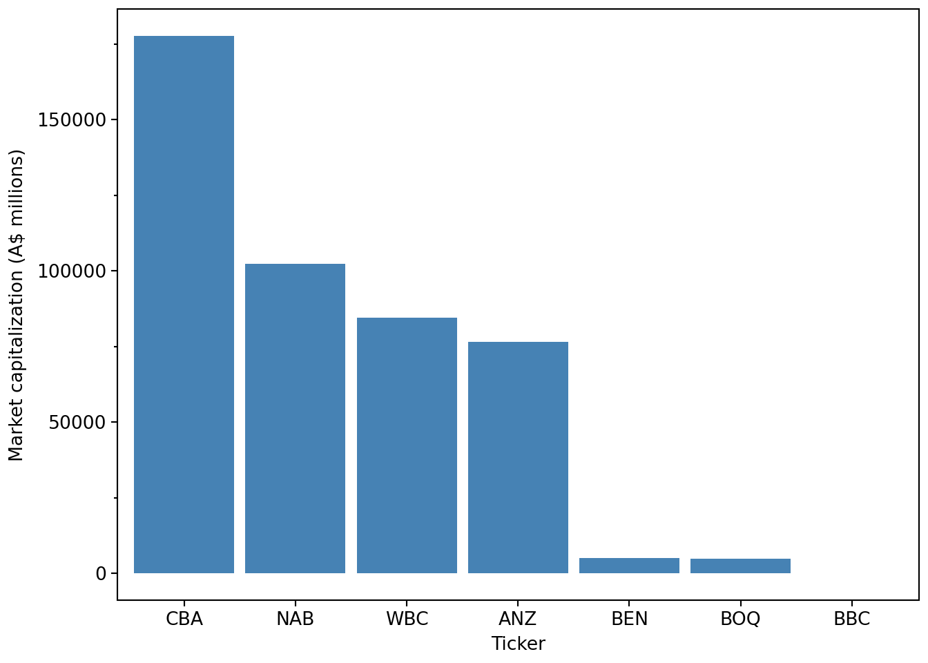
This latest_mkt_cap data frame now contains bank names and tickers and is ordered by market capitalization. These changes make it straightforward to produce a clearer plot. We also set the labels for the x- and y-axes.¹⁰

(
    latest_mkt_cap
    .ggplot(aes(x="reorder(ticker, -mkt_cap)", y="mkt_cap"))
    .geom_col(fill="steelblue")
    .labs(x="Ticker", y="Market capitalization (A$ millions)")
)

Figure 2.2: Market capitalization of Australian banks

2.5 Basic data analysis and statistics

Having covered some ground in terms of manipulating data frames and making plots in Python, we now move on to some basic statistics. Although we assume little prior knowledge of statistics, our focus in this section is on conducting statistical analysis using Python.

2.5.1 Mean

The mean of a variable \(x\) in a sample of \(n\) observations is \(\bar{x} = \frac{\sum_{i=1}^n x_i}{n}\), where \(x_i\) is the value for observation \(i\).

We can calculate the sum of a column using the .sum() method and the number of observations using .len().

aus_bank_funds.select(pl.col("ib").sum())

shape: (1, 1)

ib
f64
520938.662

So we can calculate the mean of ib “by hand” as follows:

(
    aus_bank_funds
    .select(pl.col("ib").sum() / pl.col("ib").len())
)

shape: (1, 1)

ib
f64
1840.772657

Of course, Polars provides a built-in .mean() method, which produces the same result:

aus_bank_funds.select(pl.col("ib").mean())

shape: (1, 1)

ib
f64
1840.772657

2.5.2 Missing values

At this point, we take a brief digression about missing values.

One thing you may notice in aus_bank_rets is that the first value of ret is missing. This arises because returns are calculated by comparing prices across time, and there is always a first observation for which a return cannot be computed.

Missing values also arise in many other settings, such as survey data when participants do not answer all questions, or when combining multiple data sets that do not perfectly overlap (as we will see below).

The correct handling of missing values is important in statistical analysis. To illustrate, let’s return to the data on Anne, Bertha, and Charlie from above and assume that these data were self-reported on a survey. For weights, Anne reported 51, Bertha reported 55, but Charlie did not answer the question.

survey_data = pl.DataFrame([anne, bertha, charlie])
survey_data

shape: (3, 3)

name	weight	height
str	i64	i64
"Anne"	51	null
"Bertha"	55	164
"Charlie"	null	184

In Polars, missing values are represented as null. If we ask Polars for the mean of weight, the result ignores the missing value by default:

(
    survey_data
    .select(pl.col("weight", "height").mean())
)

shape: (1, 2)

weight	height
f64	f64
53.0	174.0

Notepandas

Readers coming from pandas should note that Polars makes a clearer distinction between missing values (null) and floating-point “not a number” values (NaN).

Historically, pandas relied heavily on NumPy conventions for missing data, using values such as np.nan, None, and NaT depending on the data type. Because np.nan is a floating-point value, columns such as integers were often coerced to floating-point type when missing values were introduced.

Modern pandas has dedicated nullable data types and the scalar missing value pd.NA (introduced in version 1.0), but many users still encounter or rely on the older np.nan-based behaviour.

In Polars, .is_nan() and .is_null() are not equivalent: NaN is a floating-point value, while null represents missing data.

The default approach of Polars reflects a common practical assumption: when computing summary statistics, we often proceed using the available observations.

However, this behaviour embeds an implicit assumption that the missing observation is not systematically different from the observed ones. In the example above, if Charlie is more likely not to report his weight if he is embarrassed about his high weight, then ignoring his missing response could lead to a biased estimate of the average weight.

In some contexts, it is therefore important to be explicit about how missing values are handled. Polars allows us to detect missing values using .is_null():

In Polars, missing values are represented as null, but are entered in Python using the special value None. If we ask Polars for the mean of weight, the result ignores the missing value by default:

survey_data.select(
    pl.col("weight", "height").mean()
)

shape: (1, 2)

weight	height
f64	f64
53.0	174.0

NotePolars

Note that .filter() only keeps rows when the filter predicate evaluates to True, so both False and null values are discarded. For example, .filter(pl.col("weight") != 0) would also drop rows where weight is null. Of course, the .drop_nulls() method is more explicit: survey_data.drop_nulls(subset="weight").

2.5.3 Median and quantiles

The median of a variable can be described as its middle value. When we have an odd number of observations, the median is unambiguous.

float(np.median([1, 2, 3, 4, 5, 6, 7]))

4.0

When there is an even number of observations, the median is defined as the average of the two middle values:

float(np.median([1, 2, 3, 4, 5, 6, 7, 8]))

4.5

We can compute the median of income before extraordinary items (ib) using Polars:

aus_bank_funds.select(pl.col("ib").median())

shape: (1, 1)

ib
f64
427.0

The median is a special case of the more general idea of quantiles. In Polars, quantiles are computed using the .quantile() method:

aus_bank_funds.select(pl.col("ib").quantile(0.5))

shape: (1, 1)

ib
f64
427.0

Quantiles are expressed in terms of probabilities (so 0.5 corresponds to the 50th percentile, or median). The most commonly cited percentiles beyond the median are the 25th and 75th percentiles, also known as the first and third quartiles:

aus_bank_funds.select(
    pl.col("ib").quantile(0.25).alias("q25"),
    pl.col("ib").quantile(0.50).alias("q50"),
    pl.col("ib").quantile(0.75).alias("q75"),
)

shape: (1, 3)

q25	q50	q75
f64	f64	f64
53.791	427.0	2943.0

By default, Polars provides a convenient summary of these statistics (along with the mean, minimum, and maximum) using the .describe() method. Here, we use the .style attribute to create a formatted table from the data frame. This allows us to apply the .fmt_number() method to the ib column.

(
    aus_bank_funds
    .select("ib")
    .describe()
    .style
    .fmt_number(columns="ib", decimals=3)
)

statistic	ib
count	283.000
null_count	0.000
mean	1,840.773
std	2,565.983
min	−1,562.400
25%	53.791
50%	427.000
75%	2,943.000
max	9,928.000

The .describe() method can also be applied to an entire data frame. To select the numeric columns, we can use polars.selectors, which is usually imported as cs (for “column selectors”):

import polars.selectors as cs

(
    aus_bank_funds
    .select(cs.numeric())
    .describe()
    .style
    .fmt_number(columns=cs.numeric(), decimals=3)
)

statistic	at	ceq	ib	xi	do
count	283.000	283.000	283.000	166.000	166.000
null_count	0.000	0.000	0.000	117.000	117.000
mean	230,875.237	14,293.539	1,840.773	−31.713	−29.406
std	314,795.878	20,227.497	2,565.983	534.078	533.635
min	0.388	0.333	−1,562.400	−6,068.000	−6,068.000
25%	9,256.600	543.018	53.791	0.000	0.000
50%	76,143.100	4,980.000	427.000	0.000	0.000
75%	335,771.000	19,001.000	2,943.000	0.000	0.000
max	1,215,260.000	78,713.000	9,928.000	2,175.000	2,175.000

2.5.4 Histograms

While numerical summaries are informative, a more complete picture of a distribution is often provided by a histogram. To construct a histogram, we divide the range of values into bins, count how many observations fall into each bin, and plot these counts. In practice, we often leave most of the details to a function. We can produce a histogram of ROE values as follows:

(
    aus_bank_roes
    .ggplot(aes(x="roe"))
    .geom_histogram(bins=25)
)

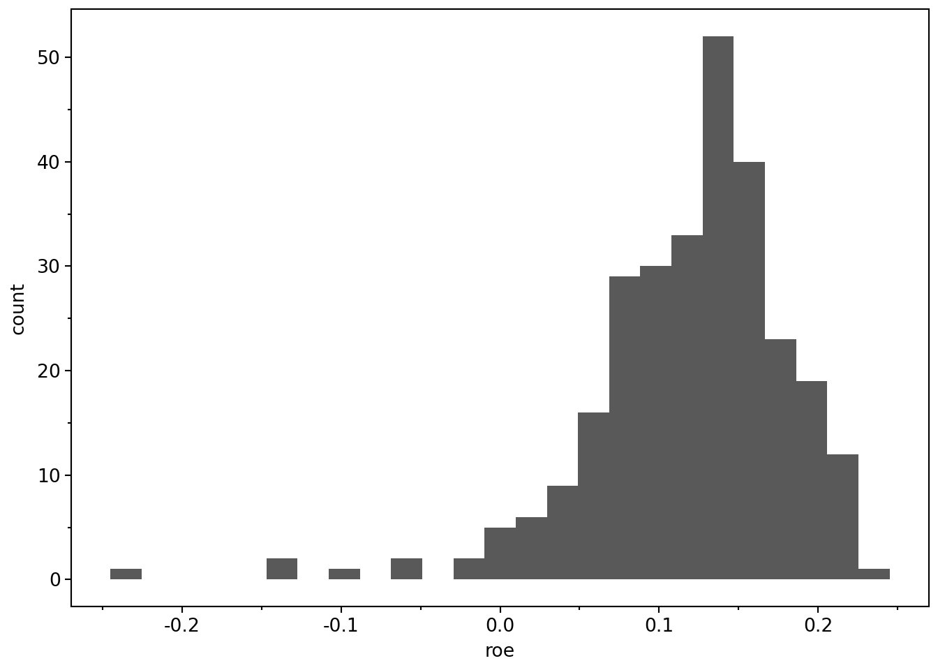
As this figure shows, most observations have positive ROE, but there is a long left tail corresponding to negative ROE firm-years.

2.5.5 Variance and standard deviation

The variance of a variable in a sample of \(n\) observations is

\[\sigma^2 = \frac{\sum_{i=1}^n (x_i - \bar{x})^2}{n - 1}, \]

where \(\bar{x}\) is the sample mean.

The denominator is \(n - 1\) rather than \(n\) for statistical reasons related to degrees of freedom. We can compute the variance of ib “by hand” using the Polars Series object.

x = aus_bank_funds["ib"].drop_nulls()
((x - x.mean()) ** 2).sum() / (len(x) - 1)

6584269.965196863

NotePolars

Like pandas, Polars allows us to access individual columns of a DataFrame as Series objects in the way we do above.

type(aus_bank_funds["ib"])

polars.series.series.Series

In some ways a Series behaves a lot like a NumPy array and offers similar methods (e.g., .mean() as used here). For reasons that will become clearer as we move to larger data sets later in the book, we generally work with columns using the pl.col() interface inside .with_columns() or .select().

Of course, Polars provides a built-in method for variance that uses the same \(n - 1\) denominator by default:

aus_bank_funds.select(pl.col("ib").var()).item()

6584269.965196864

The standard deviation is the square root of the variance:

math.sqrt(((x - x.mean()) ** 2).sum() / (len(x) - 1))

2565.9832355642666

Polars also provides a built-in method for the standard deviation:

aus_bank_funds.select(pl.col("ib").std()).item()

2565.983235564267

One benefit of the standard deviation is that it is expressed in the same units as the underlying variable (for example, dollars rather than dollars-squared).

2.5.6 Covariance and correlation

Much empirical research focuses not on how variables vary in isolation, but on how they vary together.

For example, we may be interested in how the stock returns of Australia’s two largest banks—CBA and NAB—move together over time. We begin by constructing a focused data set, rets_nab_cba, containing monthly returns for these two banks.

aus_banks

shape: (10, 3)

gvkey	ticker	co_name
str	str	str
"014802"	"NAB"	"National Australia Bank Ltd"
"015362"	"WBC"	"Westpac Banking Corp"
"015889"	"ANZ"	"ANZ Bank New Zealand Limited"
…	…	…
"203646"	"SGB"	"St. George Bank Ltd"
"212631"	"BWA"	"Bank Of Western Australia"
"312769"	"BBC"	"BNK Banking Corp Ltd"

aus_bank_rets

shape: (3_047, 4)

gvkey	datadate	ret	mkt_cap
str	date	f64	f64
"014802"	1985-12-31	null	1527.38458
"014802"	1986-01-31	0.083333	1654.666628
"014802"	1986-02-28	0.097713	1828.345559
…	…	…	…
"312769"	2022-08-31	-0.015625	74.782725
"312769"	2022-09-30	-0.111111	66.473533
"312769"	2022-10-31	0.116071	74.199628

rets_nab_cba = (
    aus_bank_rets
      .join(aus_banks, on="gvkey", how="inner")
      .filter(pl.col("ticker").is_in(["CBA", "NAB"]))
      .select("ticker", "datadate", "ret")
)

rets_nab_cba.head()

shape: (5, 3)

ticker	datadate	ret
str	date	f64
"NAB"	1985-12-31	null
"NAB"	1986-01-31	0.083333
"NAB"	1986-02-28	0.097713
"NAB"	1986-03-27	0.147727
"NAB"	1986-04-30	0.066007

2.5.7 Variance with missing values

If we compute the variance of ret across both banks combined, Polars ignores missing values by default:

rets_nab_cba.select(pl.col("ret").var())

shape: (1, 1)

ret
f64
0.003572

In practice, we are usually more interested in the variance of returns by bank. We can compute this using group_by() and aggregation:

rets_nab_cba.group_by("ticker").agg(pl.col("ret").var().alias("var_ret"))

shape: (2, 2)

ticker	var_ret
str	f64
"CBA"	0.003261
"NAB"	0.003842

2.5.8 Covariance

A central measure of how two variables vary together is covariance:

\[\mathrm{cov}(x, y) =\frac{\sum_{i=1}^n (x_i - \bar{x})(y_i - \bar{y})}{n - 1}.\]

At present, the returns for CBA and NAB appear in different rows, making covariance difficult to compute directly. We therefore reshape the data into wide form, with one column per bank.

rets_nab_cba_wide = (
    rets_nab_cba
    .filter(pl.col("ticker").is_in(["NAB", "CBA"]))
    .select("datadate", "ticker", "ret")
    .pivot(on="ticker", index="datadate", values="ret")
    .sort("datadate")
    .drop_nulls()
)

rets_nab_cba_wide.head()

shape: (5, 3)

datadate	NAB	CBA
date	f64	f64
1991-10-31	0.104972	0.106195
1991-12-31	0.054443	0.07027
1992-01-31	-0.047619	-0.075758
1992-02-28	-0.017105	0.016393
1992-03-31	-0.014726	-0.012097

With the data in this form, covariance calculations are straightforward. We can implement the covariance formula directly:

def cov_alt(x, y):
    return ((x - x.mean()) * (y - y.mean())).sum() / (pl.len() - 1)

(
    rets_nab_cba_wide
    .select(cov_alt(pl.col("NAB"), pl.col("CBA")))
    .item()
)

0.002497630122495677

The built-in Polars covariance calculation gives the same result:

(
    rets_nab_cba_wide
    .select(
        pl.cov("NAB", "CBA")
    )
    .item()
)

0.0024976301224956766

2.5.9 Correlation

A closely related concept is correlation, defined as

\[\mathrm{cor}(x, y) =\frac{\mathrm{cov}(x, y)}{\sigma_x \sigma_y},\]

where \(\sigma_x\) and \(\sigma_y\) are standard deviations.

The correlation between CBA and NAB returns is:

(
    rets_nab_cba_wide.select(
        pl.corr("NAB", "CBA").alias("corr_at_ceq")
    )
    .item()
)

0.7227703776715251

2.5.10 Linking stock prices to fundamentals

Suppose that we want to create a plot of the market-to-book ratio of each bank, where we define this ratio as mb = mkt_cap / ceq.

aus_bank_rets_sample = (
    aus_bank_rets
    .join(aus_banks, on="gvkey", how="inner")
    .filter(pl.col("ticker").is_in(latest_mkt_cap["ticker"].to_list()))
)

Clearly, we need to use one of the two-table verbs because mkt_cap is on aus_bank_rets and ceq is on aus_bank_funds.

Here is one approach:

aus_bank_mb = (
    aus_bank_rets_sample
    .join(aus_bank_funds, on=["gvkey", "datadate"], how="inner")
    .select("ticker", "datadate", "mkt_cap", "ceq")
    .sort("ticker", "datadate")
)

aus_bank_mb

shape: (145, 4)

ticker	datadate	mkt_cap	ceq
str	date	f64	f64
"ANZ"	1987-09-30	3708.075494	3138.64
"ANZ"	1988-09-30	4406.011471	3902.6
"ANZ"	1991-09-30	3924.006733	4977.7
…	…	…	…
"WBC"	2019-09-30	103441.488832	65454.0
"WBC"	2020-09-30	60820.773211	68023.0
"WBC"	2021-09-30	95383.387008	72035.0

The problem with this approach is that we have just one ratio per year. If you look at the financial pages of a newspaper or financial website, you will see that these provide values of ratios like this as frequently as they provide stock prices. They do this by comparing the latest available data for both fundamentals (here ceq) and stock prices (here mkt_cap). For example, on 28 January 2023, the website of the Australian Stock Exchange (ASX) listed a stock price for CBA of $109.85, and earnings per share of $5.415 for a price-to-earnings ratio of 20.28. The earnings per share number is the diluted earnings per share from continuing operations reported on the face of CBA’s income statement for the year ended 30 June 2022.

We can start the process of constructing something similar by using a left join (how="left") in place of the inner join (how="inner") we used above.

aus_bank_mb = (
    aus_bank_rets_sample
    .join(aus_bank_funds, on=["gvkey", "datadate"], how="left")
    .select("ticker", "datadate", "mkt_cap", "ceq")
    .sort("ticker", "datadate")
    .filter(pl.col("datadate") >= pl.date(1987, 9, 30))
)

aus_bank_mb

shape: (2_527, 4)

ticker	datadate	mkt_cap	ceq
str	date	f64	f64
"ANZ"	1987-09-30	3708.075494	3138.64
"ANZ"	1987-10-30	2708.145024	null
"ANZ"	1987-11-30	2555.377869	null
…	…	…	…
"WBC"	2022-08-31	75659.369467	null
"WBC"	2022-09-30	72263.275604	null
"WBC"	2022-10-31	84412.188702	null

The issue we see now is that most rows have no value for ceq, hence no value for mb. Following the logic applied on the ASX’s website, we want to carry forward the value of ceq until it is updated with new financial statements. In Polars, we can sort and then apply .forward_fill() within each ticker group (.over("ticker")) to produce data like the following (compare the output below with that above).¹¹

aus_bank_mb = (
    aus_bank_rets_sample
    .join(aus_bank_funds, on=["gvkey", "datadate"], how="left")
    .select("ticker", "datadate", "mkt_cap", "ceq")
    .sort("ticker", "datadate")
    .with_columns(pl.col("ceq").forward_fill().over("ticker"))
    .with_columns(mb = pl.col("mkt_cap") / pl.col("ceq"))
    .drop_nulls(subset=["mb"])
)

aus_bank_mb.filter(pl.col("datadate") >= pl.date(1987, 9, 30))

shape: (2_364, 5)

ticker	datadate	mkt_cap	ceq	mb
str	date	f64	f64	f64
"ANZ"	1987-09-30	3708.075494	3138.64	1.181427
"ANZ"	1987-10-30	2708.145024	3138.64	0.86284
"ANZ"	1987-11-30	2555.377869	3138.64	0.814167
…	…	…	…	…
"WBC"	2022-08-31	75659.369467	72035.0	1.050314
"WBC"	2022-09-30	72263.275604	72035.0	1.003169
"WBC"	2022-10-31	84412.188702	72035.0	1.171822

Now we can plot the evolution of market-to-book ratios over time, as shown in Figure 2.3.

(
    aus_bank_mb
    .ggplot(aes(x="datadate", y="mb", color="ticker"))
    .geom_line()
    .labs(x="Date", y="Market-to-Book Ratio")
)

Figure 2.3: Time-series of market-to-book for Australian banks

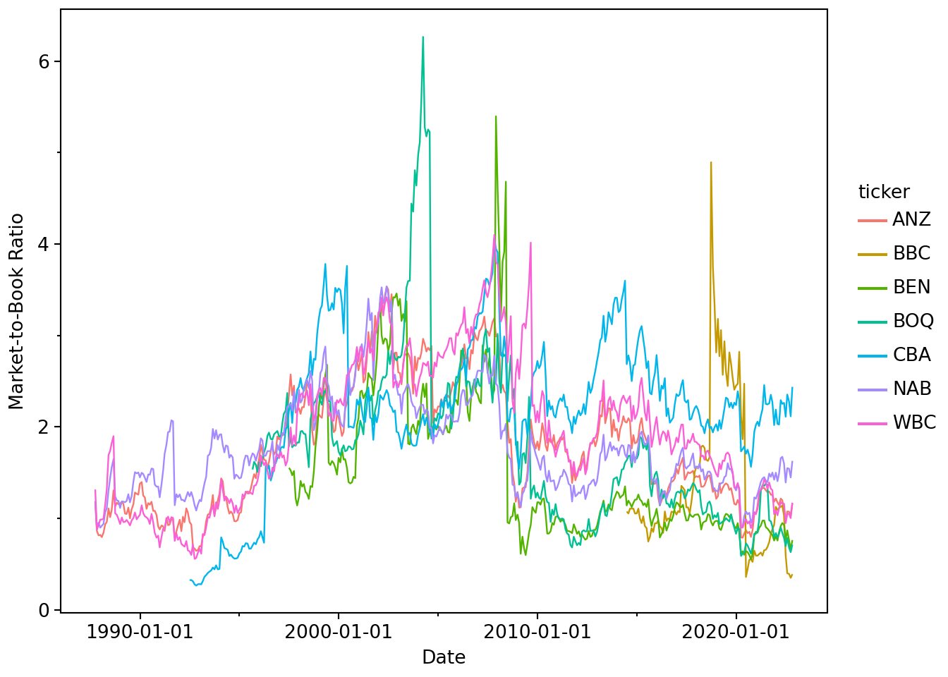
While we certainly won’t claim that Figure 2.3 is particularly insightful or “publication ready” in any sense, our hope is that the workflow above demonstrates the power of a code-based approach to data analysis.

The material above provides a very basic introduction to core ideas of Python Polars. You can learn more from the Polars documentation itself. An excellent book providing deep coverage of what Polars can do is Python Polars: The Definitive Guide by Jeroen Janssens and Thijs Nieuwdorp.

2.6 Reproducible research

A topic that has received increased attention in the research community in recent years is reproducible research. This is a complex topic and there are various ideas of what it means for research to be reproducible. One notion is that the results disseminated by a research team should be reproducible by other research teams running similar experiments. If results do not reproduce in this way, their generalizability may be questioned.

Another notion of reproducibility is more narrow. Typically results disseminated by a research team carry the implicit claim that the team took data from certain sources (sometimes these are experiments, but in accounting research, these are often from databases accessible to other researchers) and conducted certain data manipulations and statistical analyses to produce the disseminated results. The applicable notion here is that other researchers should be able to verify the data and code used to produce results, ensuring that the code functions as claimed and produces the same results. This notion of reproducibility underlies policies for sharing code and data, which will be discussed further in Chapter 19.

We bring up the issue of reproducibility so early in the course because we believe an orientation to reproducibility is a habit best formed early in one’s career. Additionally, the tools provided with modern software such as Python and R make the production of reproducible analyses easier than ever.

We also believe that reproducibility is important not only for other researchers, but also for individual researchers over time. Six months after running some numbers in Excel, you may need to explain how you got those numbers, but important steps in the analysis may have been hard-coded or undocumented. Alternatively, you might run an analysis today and then want to update it in a year’s time as more data become available (e.g., stock prices and fundamentals for the current year). If you have structured your analysis in a reproducible way, this may be as simple as running your code again. But if you copy-pasted data into Excel and used point-and-click commands to make plots, those steps would have to be repeated manually again.

Reproducibility is arguably also important for practitioners in business. For example, checking data and analysis is often a key task in auditing. Reproducible research leaves an audit trail that manual analyses do not.

Reproducibility also fosters learning and collaboration. It is much easier to get feedback from a more experienced researcher or practitioner if the steps are embedded in code. And it is much easier for collaborators to understand what you are doing and suggest ideas if they can see what you have done.

To make it easier for you to get into reproducible research, we have created Quarto templates that you can use to prepare your solutions to the exercises below. These are available on the support page for this book. For reasons of space, we do not provide details on using Quarto, but the Quarto website provides a good starting point and we direct you to other resources in the next section.

2.7 Further reading

Hopefully, the material above provides the fast-paced introduction to data analysis and visualization promised at the opening of the chapter.

Our approach in this chapter emphasizes declarative, pipeline-based data analysis, focusing on expressing what we want to do with data rather than how to do it step by step. In Python, this style is most clearly reflected in the use of tools such as Polars for data manipulation and plotnine for visualization using the grammar of graphics.

Python’s data-science ecosystem is composed of a collection of interoperating libraries. Polars provides a high-performance data-frame abstraction and tools for data manipulation, NumPy underlies much of the numerical computation, and plotting libraries such as Seaborn provide higher-level interfaces for visualization.

2.7.1 Data visualization

In accounting and finance research, data visualization appears to be relatively underutilized. We speculate that there are two main reasons for this. First, many researchers rely on tools such as Excel for plotting, which often require manual steps and make it difficult to produce reproducible visualizations. Second, data visualization is most valuable when the goal is to gain genuine insight into real-world phenomena, rather than simply to report statistically significant results. We return to this issue in more depth in Chapter 19.

We agree with the view that careful data visualization forces analysts to think clearly about the structure of their data. Throughout this book, we make frequent use of plots—not only to communicate results, but also as tools for exploration and understanding. An excellent book-length treatment of data visualization is provided by Healy (2026), which is available online.

NoteData visualization in Python

For the R edition of this book, it was relatively straightforward to choose a data visualization library. Given that that edition uses the “Tidyverse” suite of packages, ggplot2 is the natural choice. Since its release in 2005, ggplot2 has become the most widely used plotting library in R.

With Python, things are more complicated in part because Python is used for a much more diverse set of problems than R is. While Matplotlib has long been the standard library for data visualization in data science, a number of libraries have emerged to address perceived shortcomings of Matplotlib. Seaborn aims to provide “a high-level interface for drawing attractive and informative statistical graphics.” Plotnine is a package based on “the grammar of graphics, a coherent system for describing and building graphs” that uses syntax similar to ggplot2’s. Both Seaborn and Plotnine use Matplotlib as their underlying plotting engine.

The standard data visualization library for Python Polars is Altair in the sense that this package is called when one issues df.plot.scatter(). Another library offering a richer suite of plotting is hvPlot. By importing hvPlot with import hvplot.polars, one can then plot using, say, df.hvplot.scatter().

In this book, we use plotnine_polars. After import plotnine_polars, this allows us to say df.ggplot() much as one would use ggplot(df) with Plotnine in Python. One advantage of using plotnine_polars is that we can use method chains to create plots rather than having to do something like from plotnine import * to make the necessary plotting functions available.¹² Plotnine provides a higher-level plotting interface than Matplotlib and has more extensive coverage of the plots in this book than Seaborn does.

In addition to the libraries above, there are many other data visualization libraries in Python. Plotlyand Bokeh are interactive visualization libraries for browser-based graphics. Lets-Plot is a newer grammar-of-graphics library from JetBrains.

While we do strongly encourage readers to explore data visualization as part of their workflow and include plots in most chapters, we do not claim to provide a comprehensive guide to data visualization. Additionally, we emphasize more exploratory plots rather than publication-quality graphics, as the latter typically involve tweaks that would distract from our focus here.

While Healy (2026) uses R and ggplot2, almost all of the plots there can be created using plotnine with minor modifications.

We also briefly discussed reproducible research and introduced Quarto as a tool for producing reproducible analyses that combine code, output, and narrative text. Quarto supports both Python and R, as well as Jupyter notebooks, and plays a central role in the workflow used throughout this book. While we do not provide a detailed introduction to Quarto here, the Quarto website provides extensive documentation and examples.

Our expectation and hope is that, by the end of this book, you will have encountered most of the core ideas needed for modern empirical research in accounting and finance using Python. Many of these ideas—data manipulation, visualization, reproducibility, and working with relational data—are explored in greater depth in the broader data-science literature. We encourage you to consult these resources as you work through the book and to treat this chapter as a foundation on which to build more advanced skills.

2.8 Exercises

We have created Quarto templates that we recommend you use to prepare your solutions to the exercises in the book. These templates are available on the support page for this book. For this chapter, download and save py-intro.qmd.

1. Create a function var_alt(x) that uses cov_alt(x, y) to calculate the variance of x. Check that this function gives the same value as the built-in method .var() in Polars (for example, compare with rets_nab_cba_wide.select(pl.exclude("datadate").var())).

2. Create a function corr_alt(x, y) that uses cov_alt() and var_alt() to calculate the correlation between x and y. Check that it gives the same value as the built-in function in Polars (for example, compare with rets_nab_cba_wide.select(pl.corr("NAB", "CBA")).item()).

3. If you remove the .drop_nulls() line used when creating rets_nab_cba_wide, you will see missing values for CBA. There are two reasons for these missing values. One reason is explained on the Wikipedia page for Commonwealth Bank, but the other reason is more subtle and relates to how values are presented in datadate. What is the first reason? (Hint: What happened to CBA in 1991?) What is the second reason? How might you use Polars date tools to address the second reason? Does this second issue have implications for other plots?

4. Create bank_rets using the following steps:

   1. First apply either .join() or .filter() to aus_banks to focus on the banks in latest_mkt_cap.
   2. Join aus_bank_rets using .join().
   3. Normalize datadate to month-end using .dt.month_end().

   With bank_rets, .group_by() and .agg(var=pl.col("ret")), calculate the variance of returns for each bank ("ticker").

5. Create the data frame bank_rets_wide using the following steps:

   1. Apply .pivot() to bank_rets to change it from a “long” form to a “wide” form.
   2. Drop missing values using .drop_nulls().

   Correlations can also be computed for entire data frames. Calculate the correlation matrix for the returns of all banks using the following steps organized as a method chain:

   1. Drop datadate from bank_rets_wide by applying .select(pl.exclude("datadate")).
   2. Apply .corr(label="ticker") to the result.
   3. Use .with_columns(cs.numeric().round(6)) to round all numbers to six decimal places.

6. Polars does not offer a .cov() method, but pandas does. First, apply .to_pandas() and then .corr() to bank_rets_wide to check that you get the same results using pandas as you obtained in your answer to the previous question. Do you need .select(pl.exclude("datadate")) here?

   Second, use .to_pandas() and then .cov() to calculate the covariance matrix of the returns of the Australian banks. What is the calculated value of the variance of the returns for NAB?

7. From the output above, what is the value for the variance of NAB’s returns? Why does this value differ from that you calculated in response to Q1?

8. In calculating ROE above, we used ib rather than a measure of “net income”. According to WRDS, ni (net income) only applies to Compustat North America; instead use: ni = ib + xi + do. Looking at the data in aus_bank_funds, does this advice seem correct? How would you check this claim? (Hint: Focus on cases where both xi and do are non-missing; checking more recent years may be easier if you decide to consult banks’ financial statements.)

9. Figure 2.4 is a plot of market-to-book ratios. Another measure linking stock prices to fundamentals is the price-to-earnings ratio (also known as the PE ratio). Typically, PE ratios are calculated as

   \[ \textrm{PE} = \frac{\textrm{Stock price}}{\textrm{Earnings per share}} \]

   where

   \[ \textrm{Earnings per share} = \frac{\textrm{Net income}}{\textrm{Shares outstanding}} \]

   so we might write

   \[ \textrm{PE} = \frac{\textrm{Stock price} \times \textrm{Shares outstanding}}{\textrm{Net income}} \]

   What critical assumption have we made in deriving the last equation? Is this likely to hold in practice?

10. Calculating the PE ratio using pe = mkt_cap / ib, create a plot similar to Figure 2.4, but for the PE ratios of Australian banks over time.

11. Suppose you wanted to produce the plots in this chapter (market capitalization; market-to-book ratios; histogram of ROE) using Excel starting from spreadsheet versions of the three data sets provided above. Which aspects of the task would be easier? Which would be more difficult? What benefits do you see in using Python code (as we did above) rather than point-and-click tools?

Healy, K., 2026. Data visualization: A practical introduction, 2nd ed. Princeton University Press.

---

1. Unfortunately, as with any computer language, Python can be a stickler for grammar.

2. A shortcut here would be v += 4.

3. To install the numpy package, you could type pip install numpy or uv pip install numpy at the command line.

4. We discuss decimal data types in more detail in Section 7.5.

5. Note that the final example introduces a third element of the slice, step.

6. See Appendix A for more on linear algebra.

7. We can also retrieve the information using the .shape attribute.

8. The pl.date() function is a bit like the standard-library datetime.date(), but without requiring a separate import.

9. In practice, it is more common to use either average or beginning shareholders’ equity in the denominator, but this would add complexity that is unhelpful for our current purposes.

10. The figure title here is managed using Quarto code that is not visible here; see the Quarto template provided on the book’s support page for these details.

11. More advanced users might solve this problem with an as-of join rather than a left join followed by .forward_fill(). We avoid that approach given the pedagogical goals of this chapter.

12. Importing using commands like from plotnine import * is generally not recommended in Python.