6  Financial statements: A first look

In this chapter, we provide an introduction to data on financial statements, which are the primary focus of financial reporting. While a lot of contemporary accounting research has only a tangential connection to financial reporting, it’s not clear there would be a field of accounting research without financial reporting and most accounting research papers use financial reporting data to some degree (e.g., as controls). In this chapter, we will focus on annual financial statement data of North American firms, as provided by Compustat.

Tip

The code in this chapter uses the packages listed below. For instructions on how to set up your computer to use this code, go to the support page for this book. The support page also includes Quarto templates for the code and exercises below.

import polars as pl
from plotnine_polars import aes
from era_pl import load_parquet

In this chapter we start working with data sets that are much larger than the ones used in previous chapters. Rather than working with in-memory DataFrame objects, we will often work with Polars LazyFrame objects backed by local parquet data. This gives us a convenient way to work with much larger data sets, but it also means we need to think a bit more carefully about when data are actually loaded into memory. In addition, these data are not bundled with the era_pl package.

6.1 Loading WRDS data

Academic researchers generally get Compustat data through Wharton Research Data Services, more commonly referred to as WRDS (pronounced “words”).

In the Polars edition, we assume that you have created a local Parquet data repository as described on the support page for this book and that you are running the code here from a directory that includes a .env file containing DATA_DIR, which is the location of that repository on your computer.

from dotenv import load_dotenv
import os

load_dotenv()
os.getenv("DATA_DIR")

If os.getenv("DATA_DIR") does not return the expected path, Python may not be finding your .env file or it may not contain DATA_DIR. In that case, you can set DATA_DIR manually for the current session before loading data:

os.environ["DATA_DIR"] = "/path/to/your/parquet/data"

This change applies only to the current Python session. To make the setting persistent, add DATA_DIR=/path/to/your/parquet/data to the .env file in the directory from which you are running the code for this book.

Now that we have configured access to local parquet data, we can work with these data. Tables in the WRDS database is organized into schemas according to their source (in SAS, these schemas are called libraries, but we will stick with the database terminology for now).

In this chapter we focus on Compustat data, which is found in the comp schema. While there are other sources of financial statement data—especially for firms outside North America—in accounting research the pre-eminent data source is Compustat, which is typically obtained via WRDS.

We first look at the table, comp.company, which contains information about the companies in Compustat’s North American database (the equivalent table in Compustat’s “Global” database is comp.g_company). By running the following code, we create an object that points to local parquet data and behaves in many ways like the Polars data frames you have seen in earlier chapters.

company = load_parquet(table="company", schema="comp")

What have we done here? In the first line, we created an object company that points to the company table in schema comp from the local parquet library.

But what exactly is company?

One way to get information about company is to use the .show() method.

company.show()

shape: (5, 40)

conm	gvkey	add1	add2	add3	add4	addzip	busdesc	cik	city	conml	costat	county	dlrsn	ein	fax	fic	fyrc	ggroup	gind	gsector	gsubind	idbflag	incorp	loc	naics	phone	prican	prirow	priusa	sic	spcindcd	spcseccd	spcsrc	state	stko	weburl	dldte	ipodate	curr_sp500_flag
str	str	str	str	str	str	str	str	str	str	str	str	str	str	str	str	str	i16	str	str	str	str	str	str	str	str	str	str	str	str	str	i32	i32	str	str	i16	str	date	date	f64
"A & E PLASTIK PAK INC"	"001000"	null	null	null	null	null	"A & E Plastik Pak Inc. is a co…	null	null	"A & E Plastik Pak Inc"	"I"	null	"09"	null	null	"USA"	12	null	null	null	null	"D"	null	"USA"	null	null	null	null	"01"	"3089"	325	978	null	null	0	null	1978-06-30	null	0.0
"A & M FOOD SERVICES INC"	"001001"	"1924 South Utica Avenue"	null	null	null	"94104"	null	"0000723576"	"Tulsa"	"A & M Food Services Inc"	"I"	null	"01"	"73-0934497"	null	"USA"	12	"2530"	"253010"	"25"	"25301040"	"D"	null	"USA"	"722"	null	null	null	"01"	"5812"	420	978	null	"OK"	0	null	1986-07-31	null	0.0
"AAI CORP"	"001002"	"124 Industry Lane"	null	null	null	"21030-0126"	"Textron Systems Corporation de…	"0001306124"	"Hunt Valley"	"AAI Corp"	"I"	null	"01"	null	"410-628-3215"	"USA"	12	null	null	null	null	"D"	null	"USA"	null	"800 655 2616"	null	null	"01"	"3825"	230	940	null	"MD"	0	"www.textronsystems.com"	1977-03-31	null	0.0
"A.A. IMPORTING CO INC"	"001003"	"7700 Hall Street"	null	null	null	"63125"	"A.A. Importing Company, Inc. d…	"0000730052"	"St. Louis"	"A.A. Importing Co Inc"	"I"	null	"07"	"43-1232041"	"314-383-2608"	"USA"	1	"2550"	"255040"	"25"	"25504040"	"D"	"DE"	"USA"	"442110"	"314-383-8800"	null	null	"01"	"5712"	449	976	null	"MO"	3	"www.aaimporting.com"	1992-04-30	null	0.0
"AAR CORP"	"001004"	"One AAR Place, 1100 North Wood…	null	null	null	"60191"	"AAR Corp. provides products an…	"0000001750"	"Wood Dale"	"AAR Corp"	"A"	null	null	"36-2334820"	"630 227 2039"	"USA"	5	"2010"	"201010"	"20"	"20101010"	"D"	"DE"	"USA"	"423860"	"630 227 2000"	null	null	"01"	"5080"	110	925	"B"	"IL"	0	"www.aarcorp.com"	null	1972-04-24	0.0

One way to get information about company is to use the type() function.

type(company)

polars.lazyframe.frame.LazyFrame

From this, we see that company is a polars.LazyFrame (or simply LazyFrame object).¹ As a LazyFrame, the data have not yet been loaded into memory in Python, but company behaves in many important ways just like a DataFrame.

We can use .filter() to get only rows meeting certain conditions and we can use .select() to indicate which columns we want to retrieve. Finally, we can use .collect() to create a DataFrame.

(
    company
    .filter(
        pl.col("gsubind") == "45202030",
        pl.col("conm").str.slice(0, 1) == "A",
    )
    .select("gvkey", "conm", "state")
    .limit(5)
    .collect()
)

shape: (5, 3)

gvkey	conm	state
str	str	str
"001690"	"APPLE INC"	"CA"
"001820"	"ASTRONOVA INC"	"RI"
"027925"	"AVID TECHNOLOGY INC"	"MA"
"063446"	"AINOS INC"	"TX"
"324055"	"ADVANCETC LTD"	null

With lazy frames, Polars builds a query plan and executes it only when we call .collect(). We can inspect the query plan by replacing the .collect() with .explain():

(
    company
    .filter(
        pl.col("gsubind") == "45202030",
        pl.col("conm").str.slice(0, 1) == "A"
    )
    .select("gvkey", "conm", "state")
    .limit(5)
    .explain()
)

'simple π 3/3 ["gvkey", "conm", "state"]\n  SLICE[offset: 0, len: 5]\n    Parquet SCAN [/Users/igow/Dropbox/pq_data/comp/company.parquet]\n    PROJECT 4/40 COLUMNS\n    SELECTION: [([(col("conm").str.slice([dyn int: 0, dyn int: 1])) == ("A")]) & ([(col("gsubind")) == ("45202030")])]\n    ESTIMATED ROWS: 57479'

Here we see how .filter(), .select(), and .limit(5) appear in the lazy query plan as a set of instructions or a recipe for making the data.

Notepandas

The biggest conceptual shift here for pandas users is that company is not yet an in-memory data frame. It is closer to a query definition: each method adds another step to the plan, and .collect() is the moment when Polars actually executes that plan and returns a DataFrame.

While LazyFrame objects behave a lot like DataFrame objects, they are not quite the same thing and, for many purposes, we need to materialize local data frames. For example, the ols() function from StatsModels assumes that the object provided as its data argument is in-memory data (in fact, a pandas data frame). Conversion from a lazy table to an in-memory Polars data frame is achieved using .collect(). Here we use .collect() and store the result in df_company.

df_company = (
    company
    .filter(
        pl.col("gsubind") == "45202030",
        pl.col("conm").str.slice(0, 1) == "A",
    )
    .select("gvkey", "conm", "state")
    .collect()
)

Looking at type(df_company), we see that it is a pl.DataFrame.

type(df_company)

polars.dataframe.frame.DataFrame

df_company

shape: (5, 3)

gvkey	conm	state
str	str	str
"001690"	"APPLE INC"	"CA"
"001820"	"ASTRONOVA INC"	"RI"
"027925"	"AVID TECHNOLOGY INC"	"MA"
"063446"	"AINOS INC"	"TX"
"324055"	"ADVANCETC LTD"	null

NotePolars

At this point, you may be wondering why we are bothering with lazy frames at all. They seem to require an extra step (.collect()) and “lazy” doesn’t seem like something you’d want your data frames to be. We will soon explain why the LazyFrame is actually a key element of the power of Polars.

6.2 Financial statement data

Two core tables for the North American Compustat data are comp.funda, which contains annual financial statement data, and comp.fundq, which contains quarterly data.

funda = load_parquet("funda", "comp")
fundq = load_parquet("fundq", "comp")

We can get information about the columns of funda using .collect_schema().

len(funda.collect_schema())

949

From the above, we can see that comp.funda is a very wide table, with 949 columns.

We can also inspect this LazyFrame by materializing just a few rows using .show(). Because the table is so wide, we can use cs.by_index(range(6)) to select the first six columns.

import polars.selectors as cs

funda.select(cs.by_index(range(6))).show()

shape: (5, 6)

gvkey	datadate	fyear	indfmt	consol	popsrc
str	date	i32	str	str	str
"001000"	1961-12-31	1961	"INDL"	"C"	"D"
"001000"	1962-12-31	1962	"INDL"	"C"	"D"
"001000"	1963-12-31	1963	"INDL"	"C"	"D"
"001000"	1964-12-31	1964	"INDL"	"C"	"D"
"001000"	1965-12-31	1965	"INDL"	"C"	"D"

And, here we look at the next six:

funda.select(cs.by_index(range(6, 12))).show()

shape: (5, 6)

datafmt	tic	cusip	conm	acctchg	acctstd
str	str	str	str	str	str
"STD"	"AE.2"	"000032102"	"A & E PLASTIK PAK INC"	null	null
"STD"	"AE.2"	"000032102"	"A & E PLASTIK PAK INC"	null	null
"STD"	"AE.2"	"000032102"	"A & E PLASTIK PAK INC"	null	null
"STD"	"AE.2"	"000032102"	"A & E PLASTIK PAK INC"	null	"DS"
"STD"	"AE.2"	"000032102"	"A & E PLASTIK PAK INC"	null	"DS"

With so many columns, it’s a moderately large table (at the time of writing, about 1 GB in PostgreSQL), but by focusing on certain columns, the size of the data can be dramatically reduced. Let’s learn more about this table.

First, how many rows does it have?

funda.select(pl.len()).collect().item()

939537

From this snippet, we can see that comp.funda has 939,537 rows. When applied to an ungrouped frame, .len() simply counts the number of rows. In this case, we use funda.select(pl.len()) and extract the scalar count from the collected result.

While not evident from casual inspection of the table, the primary key of comp.funda is (gvkey, datadate, indfmt, consol, popsrc, datafmt). A primary key is a variable, or combination of variables, that uniquely identifies each row in a table. In other words, no two rows should share the same value of the primary key. Primary keys matter because they determine the level at which the data are recorded and because many data operations, especially joins, implicitly rely on keys being unique when uniqueness is expected. If a supposed primary key is not unique, merges can duplicate rows and produce misleading results.² That this requirement is met can be seen with output from the following code, which counts the number of rows associated with each set of values for (gvkey, datadate, indfmt, consol, popsrc, datafmt) and stores that number in num_rows and then displays the various values of num_rows.

(
    funda
    .group_by("gvkey", "datadate", "indfmt", 
              "consol", "popsrc", "datafmt")
    .agg(num_rows=pl.len())
    .group_by("num_rows")
    .agg(n=pl.len())
    .collect()
)

shape: (1, 2)

num_rows	n
u32	u32
1	939537

Because num_rows is equal to 1 in 939,537 cases and this is the number of rows in the data set, we have (gvkey, datadate, indfmt, consol, popsrc, datafmt) as a valid key.

The second requirement of a primary key is that none of its columns contains null values. This requirement is natural because a primary key is meant to identify each row uniquely, and a missing value cannot be considered a reliable identifier.³ If one component of a composite key were missing, we could no longer be sure which real-world entity or observation that row corresponds to, and joins or duplicate checks based on the key could behave in unintended ways. The code below checks this requirement.

(
    funda
    .filter(
        pl.any_horizontal(
            pl.col("gvkey", "datadate", "indfmt", 
                   "consol", "popsrc", "datafmt")
            .is_null()
        )
    )
    .select(pl.len())
    .collect()
)

shape: (1, 1)

len
u32
0

NotePolars

Note that we use the pl.any_horizontal() to evaluate a condition across multiple columns. Polars also offers functions such as pl.all_horizontal() and pl.sum_horizontal().

Notepandas

Readers coming from pandas may be used to writing row-wise checks using axis=1, for example df[key_cols].isna().any(axis=1). Polars maintains a much stronger distinction between methods that operate along rows and those that operate across columns than is implied by axis=0 versus axis=1 distinction in pandas. While this can result in more verbose code, this distinction facilitates the effeciency benefits provided by Polars.

Teasing apart the primary key, we have a firm identifier (gvkey) and financial period identifier (datadate), along with four variables that are more technical in nature: indfmt, consol, popsrc, and datafmt. Table 6.1 provides the number of observations for each set of values of these four variables.

(
    funda
    .group_by("indfmt", "consol", "popsrc", "datafmt")
    .agg(n=pl.len())
    .sort("n", descending=True)
    .collect()
)

Table 6.1: Observations by (indfmt, consol, popsrc, datafmt) values

shape: (12, 5)

indfmt	consol	popsrc	datafmt	n
str	str	str	str	u32
"INDL"	"C"	"D"	"STD"	598746
"INDL"	"C"	"D"	"SUMM_STD"	289974
"FS"	"C"	"D"	"STD"	48694
"INDL"	"P"	"D"	"STD"	1179
"INDL"	"R"	"D"	"STD"	480
…	…	…	…	…
"INDL"	"R"	"D"	"SUMM_STD"	28
"INDL"	"D"	"D"	"STD"	25
"INDL"	"D"	"D"	"SUMM_STD"	25
"INDL"	"C"	"D"	"PRE_AMENDS"	19
"INDL"	"C"	"D"	"PRE_AMENDSS"	10

As discussed on the CRSP website, the first set of values, which covers 598,746 observations, represents the standard (STD) secondary keyset, as it is what is used by most researchers when using Compustat. We can create a version of funda that limits data to this STD secondary keyset as follows:

funda_mod = (
    funda
    .filter(
        pl.col("indfmt") == "INDL",
        pl.col("datafmt") == "STD",
        pl.col("consol") == "C",
        pl.col("popsrc") == "D",
    )
)

For funda_mod, (gvkey, datadate) should represent a primary key. We can check the first requirement using code like that we used above (we already confirmed the second requirement for the larger data set).

(
    funda_mod
    .group_by("gvkey", "datadate")
    .agg(num_rows=pl.len())
    .group_by("num_rows")
    .agg(n=pl.len())
    .collect()
)

shape: (1, 2)

num_rows	n
u32	u32
1	598746

Now, let’s look at the table comp.company, which the following code confirms has 40 columns and for which gvkey is a primary key.

company.show()

shape: (5, 40)

conm	gvkey	add1	add2	add3	add4	addzip	busdesc	cik	city	conml	costat	county	dlrsn	ein	fax	fic	fyrc	ggroup	gind	gsector	gsubind	idbflag	incorp	loc	naics	phone	prican	prirow	priusa	sic	spcindcd	spcseccd	spcsrc	state	stko	weburl	dldte	ipodate	curr_sp500_flag
str	str	str	str	str	str	str	str	str	str	str	str	str	str	str	str	str	i16	str	str	str	str	str	str	str	str	str	str	str	str	str	i32	i32	str	str	i16	str	date	date	f64
"A & E PLASTIK PAK INC"	"001000"	null	null	null	null	null	"A & E Plastik Pak Inc. is a co…	null	null	"A & E Plastik Pak Inc"	"I"	null	"09"	null	null	"USA"	12	null	null	null	null	"D"	null	"USA"	null	null	null	null	"01"	"3089"	325	978	null	null	0	null	1978-06-30	null	0.0
"A & M FOOD SERVICES INC"	"001001"	"1924 South Utica Avenue"	null	null	null	"94104"	null	"0000723576"	"Tulsa"	"A & M Food Services Inc"	"I"	null	"01"	"73-0934497"	null	"USA"	12	"2530"	"253010"	"25"	"25301040"	"D"	null	"USA"	"722"	null	null	null	"01"	"5812"	420	978	null	"OK"	0	null	1986-07-31	null	0.0
"AAI CORP"	"001002"	"124 Industry Lane"	null	null	null	"21030-0126"	"Textron Systems Corporation de…	"0001306124"	"Hunt Valley"	"AAI Corp"	"I"	null	"01"	null	"410-628-3215"	"USA"	12	null	null	null	null	"D"	null	"USA"	null	"800 655 2616"	null	null	"01"	"3825"	230	940	null	"MD"	0	"www.textronsystems.com"	1977-03-31	null	0.0
"A.A. IMPORTING CO INC"	"001003"	"7700 Hall Street"	null	null	null	"63125"	"A.A. Importing Company, Inc. d…	"0000730052"	"St. Louis"	"A.A. Importing Co Inc"	"I"	null	"07"	"43-1232041"	"314-383-2608"	"USA"	1	"2550"	"255040"	"25"	"25504040"	"D"	"DE"	"USA"	"442110"	"314-383-8800"	null	null	"01"	"5712"	449	976	null	"MO"	3	"www.aaimporting.com"	1992-04-30	null	0.0
"AAR CORP"	"001004"	"One AAR Place, 1100 North Wood…	null	null	null	"60191"	"AAR Corp. provides products an…	"0000001750"	"Wood Dale"	"AAR Corp"	"A"	null	null	"36-2334820"	"630 227 2039"	"USA"	5	"2010"	"201010"	"20"	"20101010"	"D"	"DE"	"USA"	"423860"	"630 227 2000"	null	null	"01"	"5080"	110	925	"B"	"IL"	0	"www.aarcorp.com"	null	1972-04-24	0.0

First, each gvkey value is associated with just one row.

(
    company
    .group_by("gvkey")
    .agg(num_rows=pl.len())
    .group_by("num_rows")
    .agg(n=pl.len())
    .collect()
)

shape: (1, 2)

num_rows	n
u32	u32
1	57479

Second, there are no missing values of gvkey.

(
    company
    .filter(pl.col("gvkey").is_null())
    .select(pl.len())
    .collect()
)

shape: (1, 1)

len
u32
0

6.2.1 Illustration: Microsoft versus Apple

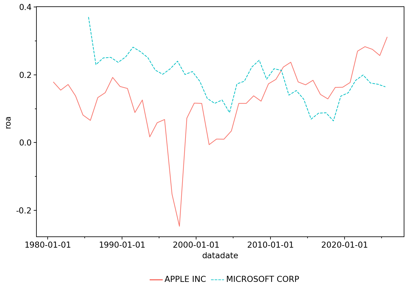
Suppose that we were interested in comparing the profitability of Apple and Microsoft over time. To measure performance, we will calculate a measure of return on assets, here measured as the value of “Income Before Extraordinary Items” scaled by “Total Assets” for Microsoft (GVKEY: 012141) and Apple (GVKEY: 001690) over time.⁴

sample = (
    company
    .filter(pl.col("gvkey").is_in(["001690", "012141"]))
    .select("conm", "gvkey")
)

sample.collect()

shape: (2, 2)

conm	gvkey
str	str
"APPLE INC"	"001690"
"MICROSOFT CORP"	"012141"

Here we can see that sample is a LazyFrame with the company name (conm) and identifier (gvkey) for Apple and Microsoft. We can use .explain() to see what this lazy query represents.

sample.explain()

'Parquet SCAN [/Users/igow/Dropbox/pq_data/comp/company.parquet]\nPROJECT 2/40 COLUMNS\nSELECTION: col("gvkey").is_in([["001690", "012141"]])\nESTIMATED ROWS: 57479'

Here .filter() and .select() appear in the plan and are only executed when we collect results.

It turns out that “Income Before Extraordinary Items” is represented by ib and “Total Assets” is at (see the CRSP manual for details). We can further restrict funda beyond funda_mod so that it contains just the key variables (gvkey, datadate) and the values for ib and at as follows. (In the following code, we will gradually refine the data set assigned to ib_at.)

ib_at = funda_mod.select("gvkey", "datadate", "ib", "at")

ib_at.limit(5).collect()

shape: (5, 4)

gvkey	datadate	ib	at
str	date	f64	f64
"001000"	1961-12-31	0.05	null
"001000"	1962-12-31	0.12	null
"001000"	1963-12-31	0.003	null
"001000"	1964-12-31	0.039	1.416
"001000"	1965-12-31	-0.197	2.31

and then restrict this by joining it with sample as follows:

ib_at = (
    funda_mod
    .select("gvkey", "datadate", "ib", "at")
    .join(sample, on="gvkey", how="inner")
)

ib_at.limit(5).collect()

shape: (5, 5)

gvkey	datadate	ib	at	conm
str	date	f64	f64	str
"001690"	2013-09-30	37037.0	207000.0	"APPLE INC"
"001690"	2015-09-30	53394.0	290479.0	"APPLE INC"
"001690"	2014-09-30	39510.0	231839.0	"APPLE INC"
"001690"	1980-09-30	11.698	65.35	"APPLE INC"
"001690"	1981-09-30	39.42	254.838	"APPLE INC"

We next calculate a value for return on assets (using income before extraordinary items and the ending balance of total assets for simplicity).

ib_at = (
    funda_mod
    .select("gvkey", "datadate", "ib", "at")
    .join(sample, on="gvkey", how="inner")
    .with_columns((pl.col("ib") / pl.col("at")).alias("roa"))
)

At this stage, ib_at is still a LazyFrame, as we can see using the type() function.

type(ib_at)

polars.lazyframe.frame.LazyFrame

To bring the data into Python, we can use .collect():

ib_at = (funda_mod
    .select("gvkey", "datadate", "ib", "at")
    .join(sample, on="gvkey", how="inner")
    .with_columns(roa=pl.col("ib") / pl.col("at"))
    .collect()
)

Now we have a pl.DataFrame:

type(ib_at)

polars.dataframe.frame.DataFrame

Note that because we have used .select() to get to just five fields and .join() to focus on two firms, the data frame ib_at is just 4 kB in size. Note the placement of .collect() at the end of this pipeline means that the amount of data we need to load into memory is quite small. If we had placed .collect() immediately after funda_mod, we would have loaded data on thousands of observations and many variables. If we had placed .collect() immediately after the .select() statement, we would have loaded data on thousands of observations, but just 4 variables. But by placing .collect() at the end of the pipeline, after both the .join() and the calculation of roa, we are only loading firm-years related to Microsoft and Apple.

Bringing data into our local Python session requires reading them off disk and loading them into memory. These operations are relatively slow, so it is worth delaying .collect() until we have narrowed the data as much as possible.

Notepandas

If you are used to pandas, it may help to think of .collect() as doing the expensive part of read_parquet(...).query(...).loc[...], except that Polars can push the filtering and projection down before materializing the result. That is why the placement of .collect() matters so much in lazy pipelines.

Having collected our data, we can make Figure 6.1.

(
    ib_at
    .ggplot(aes(x="datadate", y="roa", color="conm", linetype="conm"))
    .geom_line()
    .labs(color="", linetype="")
    .add_theme(legend_position="bottom")
)

Figure 6.1: ROA over time for Microsoft and Apple

NotePolars

A LazyFrame represents a query plan, not in-memory columns (or Series objects). So code that accesses Series such as df["col"] will work for a DataFrame, but not for a LazyFrame. While we only worked with DataFrame and not LazyFrame objects in the preceding chapters, we use .select(), .with_columns(), and pl.col() to emphasize approaches that work with both DataFrame and LazyFrame objects. Going forward, we will occasionally use Series methods with DataFrame objects when they are the most natural approach (e.g., converting a pandas pd.Series to a Polars Series when the former is returned by a function).

6.3 Exercises

1. Suppose we didn’t have access to Compustat (or an equivalent database) for the analysis above, describe a process you would use to get the data required to make the plot above comparing performance of Microsoft and Apple.

2. In the following code, how do funda_mod and funda_mod_alt differ? (For example, where are the data for each table?) What does the limit(100).collect() at the end of this code do?

funda_mod = (
    funda
    .filter(
        pl.col("indfmt") == "INDL",
        pl.col("datafmt") == "STD",
        pl.col("consol") == "C",
        pl.col("popsrc") == "D",
        pl.col("fyear") >= 1980
    )
)

funda_mod_alt = funda_mod.limit(100).collect()

3. The table comp.company has data on SIC (Standard Industrial Classification) codes in the field sic. In words, what is the when/then/otherwise logic doing in the following code? What happens if we omit .otherwise(None)? Why do we end up with just two rows?

sample = (
    company
    .select("gvkey", "sic")
    .with_columns(
        pl.when(pl.col("gvkey") == "001690")
        .then(pl.lit("Apple"))
        .when(pl.col("gvkey") == "012141")
        .then(pl.lit("Microsoft"))
        .otherwise(None)
        .alias("co_name")
    )
    .filter(pl.col("co_name").is_not_null())
)

4. What does the data frame another_sample represent? Why do we use .filter(pl.col("gvkey") != pl.col("gvkey_right"))?

another_sample = (
    company
    .select("gvkey", "sic")
    .join(sample, on="sic", how="inner", suffix="_right")
    .filter(pl.col("gvkey") != pl.col("gvkey_right"))
    .with_columns(group=pl.col("co_name") + " peer")
    .select("gvkey", "group")
)

5. What is the following code doing?

total_sample = pl.concat(
    [
        sample
        .with_columns(group=pl.col("co_name"))
        .select("gvkey", "group"),
        another_sample,
    ],
    how="vertical",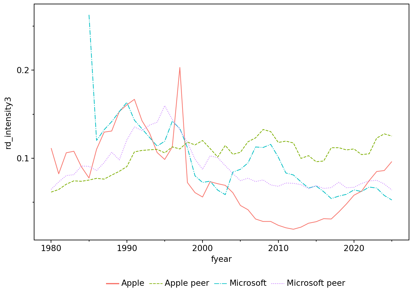
)

6. Suppose that we are interested in firms’ R&D activity. One measure of R&D activity is R&D Intensity, which can be defined as “R&D expenses” (Compustat item xrd) scaled by “Total Assets” (Compustat item at). In xrd_at, what’s the difference between rd_intensity and rd_intensity_alt? Does .filter(pl.col("at") > 0) seem like a reasonable filter? What happens if we omit it?

xrd_at = (
    funda_mod
    .select("gvkey", "datadate", "fyear", "conm", "xrd", "at")
    .filter(pl.col("at") > 0)
    .with_columns(
        rd_intensity=pl.col("xrd") / pl.col("at"),
        xrd_alt=pl.col("xrd").fill_null(0),
        rd_intensity_alt=pl.col("xrd").fill_null(0)
            / pl.col("at"),
    )
    .join(total_sample, on="gvkey", how="inner"))

7. Looking at a sample of rows from xrd_at_sum, it appears that the three R&D intensity measures are always identical for Apple and Microsoft, but generally different for their peer groups. What explains these differences? Can you say that one measure is “correct”? Or would you say “it depends”?

xrd_at_sum = (
    xrd_at
    .group_by("group", "fyear")
    .agg(
        rd_intensity1=(pl.col("xrd") / pl.col("at")).mean(),
        rd_intensity2=(pl.col("xrd_alt") / pl.col("at")).mean(),
        rd_intensity3=pl.when(pl.col("at").sum() > 0)
            .then(pl.col("xrd").sum() / pl.col("at").sum()),
    )
    .collect()
)

(
    xrd_at_sum
    .sort(["fyear", "group"], 
          descending=[True, False])
    .limit(8)
)

shape: (8, 5)

group	fyear	rd_intensity1	rd_intensity2	rd_intensity3
str	i32	f64	f64	f64
"Apple"	2025	0.096175	0.096175	0.096175
"Apple peer"	2025	0.101371	0.093862	0.125179
"Microsoft"	2025	0.052484	0.052484	0.052484
"Microsoft peer"	2025	0.155815	0.131026	0.06377
"Apple"	2024	0.08595	0.08595	0.08595
"Apple peer"	2024	0.141817	0.137646	0.127616
"Microsoft"	2024	0.057618	0.057618	0.057618
"Microsoft peer"	2024	0.30382	0.250908	0.070659

8. Write code to produce Figure 6.2. Also produce plots that use rd_intensity1 and rd_intensity2 as measures of R&D intensity. Do the plots help you think about which of the three measures makes most sense? (Hint: The data are in xrd_at_sum.)

Figure 6.2: R&D intensity over time for Microsoft and Apple and their peers

6.4 Appendix: Loading Parquet data into Polars

You might wonder what the function load_parquet() from the era_pl package is doing. In essence, it is calling the function pl.scan_parquet() to load a Parquet file named table.parquet located in the schema directory under DATA_DIR:

import os
from pathlib import Path

def load_parquet(table, schema, data_dir=None):
    if data_dir is None:
        data_dir = os.getenv("DATA_DIR")
    
    data_dir = Path(data_dir).expanduser()
    pq_path = data_dir / schema / f"{table}.parquet"
    return pl.scan_parquet(pq_path)

company = load_parquet(table="company", schema="comp")

The function pl.scan_parquet() lazily reads from a Parquet file to create a pl.LazyFrame, while the function pl.read_parquet() eagerly reads data from a Parquet file to create a pl.DataFrame.

The other era_pl function we have used to get data—load_data()—actually uses pl.read_parquet() behind the scenes to read Parquet files stored inside that package.

---

1. You probably see something like polars.lazyframe.frame.LazyFrame, but we will use LazyFrame in this book for reasons of brevity.

2. Chapter 19 of R for Data Science discusses this point.

3. For example, if gvkey is a firm identifier and a candidate primary key, then null in gvkey means “unknown”.

4. Financial analysts might object to using an end-of-period value as the denominator; we do so here because it simplifies the coding and our goal here is just illustrative.