import polars as pl
import polars.selectors as cs
import numpy as np
import pyfixest as pf
from scipy import stats
from plotnine_polars import aes

from era_pl import (
    fit_test_score_panel, get_idd_periods, get_test_scores, load_data,
    load_parquet, ptime
)21 Panel data
The typical data set used in accounting research comprises panel data, i.e., repeated observations on multiple units. Typically units are companies and observations are available for several points of time or periods. As we saw in Chapter 3, in certain conditions, researchers can exploit panel data sets to gain insights into causal effects.
In this chapter, we explore two approaches commonly used with panel data sets. The first approach uses difference in differences to measure causal effects. The second approach uses multi-way fixed effects to account both for what is commonly referred to as “unobserved time-invariant heterogeneity” between units (i.e., unit-specific effects) and period-specific effects. In practice, these approaches are often combined. We discussed difference in differences in Chapter 19 and recommend that you read that chapter before this one.
Tip
The code in this chapter uses the packages listed below. For instructions on how to set up your computer to use this code, go to the support page for this book. The support page also includes Quarto templates for the code and exercises below.
21.1 Analysis of simulated data
In Chapter 3, we explored the test_scores data set.
There we used a number of approaches, including one where we estimated the effect size using a difference-in-differences estimator with grade and individual fixed effects as 15.73578.
We can now reveal that the test_scores and camp_attendance data sets were simulated using the function get_test_scores(), with the default values for each of its arguments: effect_size = 15, n_students = 1000, and n_grades = 4.1
The data-generating process embedded in get_test_scores() produces scores using the following equation:
\[
y_{ig} = \alpha_i + \beta x_{ig} + \gamma_g + \epsilon_{ig}
\] where \(i\) and \(g\) denote individuals and grades, respectively. Denoting the grade after application of treatment (i.e., 7 in the test_scores data) as \(G\), the treatment indicator \(x_{ig}\) is as follows:
\[ x_{ig} = \begin{cases} 1 \text{ if } i \text{ is treated and } g \geq G \\ 0 \text{ otherwise} \end{cases} \]
Thus, as we will see, this is precisely the setting where multi-way fixed effects are appropriate. The individual fixed effect picks up \(\alpha_i\) and the grade fixed effect picks up \(\gamma_g\).
The estimated effect size of 15.73578 seems close to the true value \(\beta = 15\), but is it close enough?
To better examine this issue, we generate a version of the data where the treatment effect is zero (i.e., \(\beta = 0\)).
test_scores_alt = get_test_scores(effect_size=0, seed=442)We then estimate regressions with grade- and individual-level fixed effects. One regression uses “OLS” standard errors, the other uses standard errors clustered by grade and id (see Section 5.6 for discussion of alternative approaches to calculating standard errors).
fms = [
    pf.feols(
        "score ~ I(treat * post) | grade + id",
        data=test_scores_alt,
        vcov="iid",
    ),
    pf.feols(
        "score ~ I(treat * post) | grade + id",
        data=test_scores_alt,
        vcov={"CRV1": "grade + id"},
    ),
]
Because we set the seed to the same value (442) as used to generate the original data, we get the same random draws and our estimated treatment effect is exactly as before (0.736), but reduced by \(15\) and the estimated standard error (without clustering) is exactly as we saw earlier (0.312). However, in Table 21.1, we see evidence that the coefficient is not “close enough” to the true value, as we would reject the true null at the 5% level (p-value of 0.018).
pf.etable(
    fms,
    signif_code=[0.01, 0.05, 0.1],
    custom_model_stats={"SE type": ["OLS", "CL-2"]},
)| score | ||
|---|---|---|
| (1) | (2) | |
| coef | ||
| I(treat * post) | 0.736 (0.312) |
0.736 (0.811) |
| fe | ||
| id | x | x |
| grade | x | x |
| stats | ||
| SE type | OLS | CL-2 |
| Observations | 4,000 | 4,000 |
| R2 | 0.924 | 0.924 |
| Format of coefficient cell: Coefficient (Std. Error) | ||
What has “gone wrong” in this case? Some possible explanations are:
- Our standard errors are too low.
- We had bad luck (i.e., we don’t expect similar results for a different seed value).
- Our fixed-effects estimator is biased due to its small-sample properties.
- Our estimator is biased due to endogenous selection.
Let’s take these explanations one at a time. For the first, the fact that cluster-robust standard errors are significantly higher than OLS standard errors seems consistent with this explanation. But recall that the standard error is essentially an estimate of the standard deviation of the relevant coefficient over independent random draws of the data. So a more rigorous way to test this explanation is to simulate the data and examine whether the OLS standard errors tend to underestimate the variability of the coefficients. To keep the simulation fast, we use fit_test_score_panel() from era_pl, which is a chapter-specific implementation of the test-score regression that reproduces the key outputs we use from pf.feols().
def sim_run(i: int, **kwargs) -> pl.DataFrame:
    df = get_test_scores(effect_size=0, seed=i, **kwargs)
    return pl.concat(
        [
            fit_test_score_panel(df, vcov="iid").with_columns(
                model=pl.lit("OLS")
            ),
            fit_test_score_panel(
                df, vcov={"CRV1": "grade + id"}
            ).with_columns(model=pl.lit("CL-2")),
        ],
        how="vertical",
    )
The following code runs sim_run() 1,000 times and stores the results in sim_results.
num_sims = 1000
with ptime():
    sim_results = pl.concat([sim_run(i)
                             for i in range(num_sims)],
                            how="vertical")
Wall time: 2.867 s
Given these data, we want to compare the standard deviation of the estimated coefficient with the mean of the estimated standard error for the two approaches ("OLS" and "CL-2"):
sim_results_summary = (
    sim_results
    .group_by("model")
    .agg(
        pl.col("estimate").std().alias("se_obs"),
        pl.col("se").mean().alias("se_est"),
    )
    .sort("model")
)

sim_results_summary
shape: (2, 3)
| model | se_obs | se_est |
|---|---|---|
| str | f64 | f64 |
| "CL-2" | 0.319958 | 0.999016 |
| "OLS" | 0.319958 | 0.315467 |
We can see that the two-way cluster-robust standard errors are actually far too high, while the OLS standard errors are pretty close to the true standard deviation of the coefficients. This seems to rule out the first explanation.
To evaluate the second explanation (“bad luck”), we can use the same data. Let’s consider critical p-values of 1% and 5% and count how many of the OLS test statistics would lead to rejection of the null hypothesis (\(\beta = 0\)) at each size. (We focus on the “OLS” t-statistics, as we have established that OLS produces better standard error estimates.)
rejection_stats = (
    sim_results
    .filter(pl.col("model") == "OLS")
    .select(
        (pl.col("p_value") <= 0.01).mean().alias("prop_01"),
        (pl.col("p_value") <= 0.05).mean().alias("prop_05"),
    )
)

rejection_stats
shape: (1, 2)
| prop_01 | prop_05 |
|---|---|
| f64 | f64 |
| 0.87 | 0.957 |
So, we reject a true null hypothesis \(87.00\%\) of the time at the \(1\%\)-level and \(95.70\%\) of the time at the \(5\%\)-level, even with what appear to be good standard errors.
This would be an extraordinary degree of bad luck, suggesting that there is bias in our coefficient estimates.
The properties of fixed-effect estimators are derived asymptotically, that is as the number of observations and estimated fixed effects approaches infinity. However, in a typical panel data set, we have a fairly small number of time periods. In our analysis above, we have just four grades of data. But, because these are simulated data and not real people, we can easily expand the number of grades of data that we consider. Let’s consider n_grades = 12, the maximum handled by get_test_scores().2
sim_results_wide = pl.concat(
    [sim_run(i, n_grades=12) for i in range(num_sims)],
    how="vertical",
)
We collect data on rejection rates for both \(\alpha = 0.01\) and \(\alpha = 0.05\). Based on our analysis above, we focus on the "OLS" model.
rejection_stats = (
    sim_results_wide
    .filter(pl.col("model") == "OLS")
    .select(
        (pl.col("p_value") <= 0.01).mean().alias("prop_01"),
        (pl.col("p_value") <= 0.05).mean().alias("prop_05"),
    )
)

rejection_stats
shape: (1, 2)
| prop_01 | prop_05 |
|---|---|
| f64 | f64 |
| 0.338 | 0.565 |
Here we see evidence of a reduction of the bias, but the bias is not eliminated. We still reject a true null hypothesis \(33.80\%\) of the time at the \(1\%\)-level and \(56.50\%\) of the time at the \(5\%\)-level.
So let’s consider the final explanation of the bias, which is due to non-random selection. It turns out that assignment to treatment in get_test_scores() depends on test scores in the year prior to the camp, but conditional on these scores is completely random.3 This is termed selection on observables, which is often suggested as a basis on which causal inference can be justified when using approaches such as propensity-score matching.
So what happens if we use completely random assignment to treatment? We can request such assignment by setting random_assignment=True in get_test_scores().
sim_results_rand = pl.concat(
    [sim_run(i, random_assignment=True) for i in range(num_sims)],
    how="vertical",
)
rejection_stats = (
sim_results_rand
.filter(pl.col("model") == "OLS")
.select(
(pl.col("p_value") <= 0.01).mean().alias("prop_01"),
(pl.col("p_value") <= 0.05).mean().alias("prop_05"),
)
)
rejection_stats
shape: (1, 2)
| prop_01 | prop_05 |
|---|---|
| f64 | f64 |
| 0.005 | 0.049 |
Here we see evidence of elimination of the bias. We reject a true null hypothesis \(0.50\%\) of the time at the \(1\%\)-level and \(4.90\%\) of the time at the \(5\%\)-level.
Thus, it appears that random assignment is critical in this setting for achieving valid causal inferences. This is somewhat concerning as, beyond non-random treatment assignment, the basic assumptions underlying causal inference appear to be satisfied, as we have a plausible basis for the parallel trends assumption. First, we have grade effects that are the same for both treated and untreated observations. Second, we have individual effects that, while different between the treated and untreated observations, remain constant over the sample period and therefore do not undermine the parallel-trends assumption.4 What this suggests is that subtle biases can enter difference-in-differences analyses even in settings that are unrealistically simple. It seems reasonable to expect that biases exist—and are plausibly worse—in more complex settings of actual research.
21.1.1 Exercises
Generate a random sample of test scores using
get_test_scores()with some value ofeffect_sizeand some value ofseed. Assign this to the variabledf_1. Estimate the model"score ~ I(treat * post) | grade + id"usingpf.feols()withdata=df_1andvcov="iid"and store the result infm. Compare the output offm.tidy()with that fromfit_test_score_panel(df_1, vcov="iid"). What do you observe?Estimate the model
"score ~ I(treat * post) | grade + id"usingpf.feols()withdata=df_1andvcov={"CRV1": "grade + id"}and store the result infm2. Compare the output offm2.tidy()with that fromfit_test_score_panel(df_1, vcov={"CRV1": "grade + id"}). What do you observe?Given the above, why do you think we included
fit_test_score_panel()rather than usingpf.feols()? Develop and run a test of your hypothesis for why we did so.
21.2 Voluntary disclosure
One paper that uses a multi-way fixed-effect structure like that we analysed above is Li et al. (2018), who “seek to provide causal evidence on the proprietary cost hypothesis” (2018, p. 266). While “proprietary costs” are commonly assumed to be those caused by use of information by competitors, Verrecchia (1983, p. 181) uses the term more broadly.
Many researchers focus on settings where firms want to disclose favourable information to investors. For example, Verrecchia (1983, p. 181) writes of the “proprietary cost associated with releasing information which is unfavorable to a firm (e.g., a bank would be tempted to ask for repayment of its loan).” However, Verrecchia (1983, p. 182) points out that in some situations firms may prefer to disclose bad news: “One recent example of this is the response of the UAW (United Auto Workers) for fewer labor concessions in the face of an announcement by Chrysler Corporation’s chairman that that firm’s fortunes had improved.”
While Verrecchia (1983) considers the “reluctance of managers in certain highly competitive industries … to disclose favorable accounting data”, in his model, he assumes that the cost of disclosure is constant and independent of the disclosed value.
Verrecchia (1983) can be viewed as providing a theoretical foundation for the proprietary cost hypothesis. The model in Verrecchia (1983) posits a capital market-driven incentive for disclosure of favourable information; without such an incentive, there would be no disclosure in the Verrecchia (1983) setting. Also in Verrecchia (1983), the firms with favourable news are the ones disclosing, as they have the greater capital-market benefit from doing so.
Li et al. (2018) exploit the staggered implementation of the inevitable disclosure doctrine (IDD), which was adopted by state courts as part of the common law of their respective states at different times (some state courts later rejected the doctrine after adopting it). IDD provides an employer with injunctive relief to prevent a current or former employee from working for another company if doing so will lead to the inevitable disclosure of trade secret information. Li et al. (2018) argue that IDD increases the marginal benefits of non-disclosure, which they interpret as an increase in the cost of disclosure.
Li et al. (2018) focus their analysis of disclosure choice on the disclosure of customer identities in 10-Ks and assume that the state of a firm’s headquarters governs the applicability of IDD to the firm. We will conduct an approximate replication of certain analyses of Li et al. (2018) to understand the empirical approaches of this chapter. This requires combining data on customer disclosures with data on the states of companies’ headquarters. This data set is then combined with data on the dates of adoption of IDD by states.
21.2.1 Customer disclosures
We will use three data sets in the replication analysis. The first data set is compseg.seg_customer, which contains data derived from companies’ disclosures regarding significant customers. We use the second (compseg.names_seg) to link companies on Compustat with CIKs, which we use to link with data on headquarters locations. Finally, we use comp.funda for data on total sales.
seg_customer = load_parquet("seg_customer", "compseg")
names_seg = load_parquet("names_seg", "compseg")
funda = load_parquet("funda", "comp")
It turns out that compseg.seg_customer contains data on a number of different types of segment, including geographic regions and markets.
(
    seg_customer
    .group_by("ctype")
    .agg(pl.len().alias("n"))
    .sort("n", descending=True)
    .collect()
)
shape: (7, 2)
| ctype | n |
|---|---|
| str | u32 |
| "COMPANY" | 391235 |
| "GEOREG" | 169507 |
| "MARKET" | 120263 |
| "GOVDOM" | 40620 |
| "GOVFRN" | 5135 |
| "GOVSTATE" | 1562 |
| "GOVLOC" | 586 |
We are interested in data in "COMPANY" segments, which may or may not name individual customers.
(
    seg_customer
    .filter(pl.col("ctype") == "COMPANY")
    .group_by("cnms")
    .agg(pl.len().alias("n"))
    .sort("n", descending=True)
    .collect()
)
shape: (45_760, 2)
| cnms | n |
|---|---|
| str | u32 |
| "Not Reported" | 79751 |
| "NOT REPORTED" | 31162 |
| "2 Customers" | 6602 |
| "3 Customers" | 5834 |
| "5 Customers" | 5116 |
| … | … |
| "MAGNES ELCTRN" | 1 |
| "China Ministry of Land Resourc… | 1 |
| "Esprit Pharma Inc" | 1 |
| "Transportadora de Gas del Sur … | 1 |
| "LDC Ventures Inc" | 1 |
To better understand this setting, we examine one example chosen somewhat at random from the last year of the sample period. In its 10-K for the year ended 31 December 2010, Advanced Micro Devices, Inc. (AMD), a global semiconductor company, disclosed the following:
In 2010, Hewlett-Packard Company accounted for more than 10% of our consolidated net revenues. Sales to Hewlett-Packard consisted primarily of products from our Computing Solutions segment. Five customers, including Hewlett-Packard, accounted for approximately 55% of the net revenue attributable to our Computing Solutions segment. In addition, five customers accounted for approximately 46% of the net revenue attributable to our Graphics segment. A loss of any of these customers could have a material adverse effect on our business.
Elsewhere in its 10-K, AMD discloses the following:
In 2010, the Company had one customer that accounted for more than 10% of the Company’s consolidated net revenues. Net sales to this customer were approximately $1.4 billion, or 22% of consolidated net revenues, and were primarily attributable to the Computing Solutions segment.
Note that the Graphics and Computing Solutions segments had sales of $1,663 million and $4,817 million, respectively, and therefore made up 99.8% of AMD’s total sales of $6,494 million.
Thus, 46% of Graphics represents $765 million, while 55% of Computing Solutions is $2,650 million. After subtracting $1,400 million of these sales to Hewlett-Packard (HP), Compustat appears to ascribe the remaining $1,250 to “4 Customers”. The basis for assigning $1400 to “Not Reported” is unclear (while the sentence above merely says “one customer”, it is quite clear that this is HP and Compustat elsewhere assumes as much). (In fact, it seems almost certain that there is double-counting in this case, making addition of the numbers in salecs problematic.)
(
    seg_customer
    .filter(
        pl.col("gvkey") == "001161",
        pl.col("datadate") == pl.date(2010, 12, 31),
    )
    .select("cnms", "ctype", "salecs", "stype")
    .collect()
)
shape: (8, 4)
| cnms | ctype | salecs | stype |
|---|---|---|---|
| str | str | f64 | str |
| "HEWLETT-PACKARD CO" | "COMPANY" | 1400.0 | "BUSSEG" |
| "4 Customers" | "COMPANY" | 1249.53 | "BUSSEG" |
| "Not Reported" | "COMPANY" | 1400.0 | "BUSSEG" |
| "5 Customers" | "COMPANY" | 765.0 | "BUSSEG" |
| "Not Reported" | "COMPANY" | null | "BUSSEG" |
| "Not Reported" | "COMPANY" | null | "BUSSEG" |
| "Not Reported" | "COMPANY" | null | "BUSSEG" |
| "International" | "GEOREG" | 5714.72 | "BUSSEG" |
Focusing on this case perhaps helps us to understand the disclosure decision faced by AMD. Even if AMD had not disclosed the identity of its largest customer, it perhaps would have been easy to infer that “Customer #1” was indeed HP, as HP was the largest personal computer manufacturer at the time.5
The second data set we use is undisclosed_names, which contains the values of cnms considered to be non-disclosures and is part of the era_pl package.6
undisclosed_names = load_data("undisclosed_names")
undisclosed_names
shape: (460, 2)
| cnms | disclosed |
|---|---|
| str | bool |
| "Not Reported" | false |
| "NOT REPORTED" | false |
| "2 CUSTOMERS" | false |
| "6 Customers" | false |
| "4 Customers" | false |
| … | … |
| "Nott Reported" | false |
| "NOTE REPORTED" | false |
| "NO REPORTED" | false |
| "No Reported" | false |
| "Undisclosed partner" | false |
We can then perform a left join of the customer-related data in seg_customer to identify disclosures (and non-disclosures) of customer identities. Following Li et al. (2018), we focus on the period from 1994 to 2010.
sample_start = pl.date(1994, 1, 1)
sample_end = pl.date(2010, 12, 31)

disclosure_raw = (
    seg_customer
    .filter(pl.col("ctype") == "COMPANY",
            pl.col("datadate").is_between(sample_start,
                                          sample_end))
    .collect()
    .join(undisclosed_names, on="cnms", how="left")
    .with_columns(
        pl.col("disclosed").fill_null(True)
    )
    .select("gvkey", "datadate", "cnms", "salecs", "disclosed")
)
Table 21.2 lists the largest disclosed customers in the data. Many of these observations relate to Walgreens and CVS, two large US pharmacy chains.
(
    disclosure_raw
    .filter(pl.col("disclosed"))
    .sort("salecs", descending=True, nulls_last=True)
    .select("gvkey", "datadate", "cnms", "salecs")
    .head(10)
    .style
    .fmt_integer(columns="salecs")
)| gvkey | datadate | cnms | salecs |
|---|---|---|---|
| 002751 | 2010-06-30 | CVS Health Corp | 23,641 |
| 002751 | 2009-06-30 | WALGREEN CO | 22,888 |
| 118122 | 1999-12-31 | General Motors Corp | 22,302 |
| 002751 | 2010-06-30 | WALGREEN CO | 21,671 |
| 002751 | 2009-06-30 | CVS Caremark Corp | 20,898 |
| 118122 | 2000-12-31 | General Motors Corp | 20,665 |
| 002751 | 2008-06-30 | CVS Caremark Corp | 20,040 |
| 002751 | 2007-06-30 | CVS Caremark Corp | 18,239 |
| 012136 | 2005-06-30 | GENERAL ELECTRIC CO | 17,712 |
| 002751 | 2008-06-30 | Walgreen Co | 17,307 |
As a shortcut way of imposing the sample requirements used in Li et al. (2018) (e.g., not financial services), we restrict our analysis to firms (GVKEYs) in the sample of Li et al. (2018). The llz_2018 data set from the era_pl package contains these GVKEYs.7
To get a feel for the data, we calculate the proportion of total sales that are made to the largest disclosed customer.
sales = (
funda
.filter(
pl.col("indfmt") == "INDL",
pl.col("datafmt") == "STD",
pl.col("consol") == "C",
pl.col("popsrc") == "D",
)
.select("gvkey", "datadate", "sale")
.collect()
)
biggest_customers = (
disclosure_raw
.filter(pl.col("disclosed"))
.join(sales, on=["gvkey", "datadate"], how="inner")
.filter(
pl.col("sale").is_not_null(),
pl.col("salecs").is_not_null(),
pl.col("sale") > 0,
)
.group_by("gvkey", "datadate")
.agg(
(pl.col("salecs").max() / pl.col("sale").first()).alias(
"max_customer"
)
)
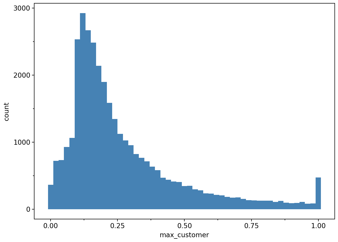
)Figure 21.1 provides a look at the proportion of sales attributed to the largest disclosed customer. Note that there are some cases where the largest customer appears to account for more than 100% of sales; many of these appear to be data-entry errors. But there are hundreds of firm-years with revenue from just one customer.
There is also an interesting jump at 10% of sales. While this is likely driven by the 10% cutoff for mandatory disclosure, interestingly many firms disclose significant customer information even when the largest customer is below 10% of sales, as seen in Figure 21.1.
(
    biggest_customers
    .filter(pl.col("max_customer").is_between(0, 1))
    .ggplot(aes(x="max_customer"))
    .geom_histogram(binwidth=0.02, fill="steelblue")
)
Interestingly, Li et al. (2018) only include firm-year observations where at least one customer is disclosed (whether identified or not) as having at least 10% of total sales. We construct a data set (prin_custs) to identify these firms.
prin_custs = (
    disclosure_raw
    .join(sales, on=["gvkey", "datadate"], how="inner")
    .filter(pl.col("salecs").is_not_null(),
            pl.col("sale") > 0)
    .group_by("gvkey", "datadate")
    .agg(
        (pl.col("salecs").max() / pl.col("sale").first())
        .alias("prin_cust")
    )
    .with_columns(has_prin_cust=pl.col("prin_cust") >= 0.1)
)
We next restrict the data to the llz_2018 sample and calculate the two measures of disclosure choice used in Li et al. (2018), one measuring the proportion of significant customers whose identities are not disclosed and another weighting that proportion by sales.
llz_2018 = load_data("llz_2018")

disclosure = (
    disclosure_raw
    .join(sales, on=["gvkey", "datadate"], how="inner")
    .join(llz_2018, on="gvkey", how="inner")
    .group_by("gvkey", "datadate")
    .agg(
        pl.col("disclosed").not_().mean().alias("ratio"),
        pl.when(pl.col("salecs").is_null().any())
        .then(None)
        .otherwise(
            (pl.col("disclosed").not_().cast(pl.Float64) * pl.col("salecs")).sum()
            / pl.col("salecs").sum()
        ).alias("ratio_sale"),
    )
    .with_columns(year=pl.col("datadate").dt.year())
)
Table 21.3 provides summary statistics for the two measures of disclosure choice. These are fairly similar to those disclosed in Li et al. (2018) (e.g., Panel C of Table 1 reports a mean of 0.447 for Ratio 1, the measure we call ratio).
(
    disclosure
    .select("ratio", "ratio_sale")
    .unpivot(variable_name="measure", value_name="value")
    .group_by("measure")
    .agg(
        pl.col("value").mean().alias("mean"),
        pl.col("value").median().alias("median"),
        pl.col("value").std().alias("sd"),
    )
    .sort("measure")
    .style
    .fmt_number(columns=cs.numeric(), decimals=3)
)| measure | mean | median | sd |
|---|---|---|---|
| ratio | 0.459 | 0.333 | 0.449 |
| ratio_sale | 0.461 | 0.316 | 0.465 |
21.2.2 Data on adoption of IDD
The next data set we use is idd_periods, which is returned by get_idd_periods(). This function relies on idd_dates, a data set in the era_pl package derived from data reported in Klasa et al. (2018) and reproduced in Li et al. (2018).
idd_dates = load_data("idd_dates")
idd_dates
shape: (24, 3)
| state | idd_date | idd_type |
|---|---|---|
| str | date | str |
| "AR" | 1997-03-18 | "Adopt" |
| "CT" | 1996-02-28 | "Adopt" |
| "DE" | 1964-05-05 | "Adopt" |
| "FL" | 1960-07-11 | "Adopt" |
| "FL" | 2001-05-21 | "Reject" |
| … | … | … |
| "PA" | 1982-02-19 | "Adopt" |
| "TX" | 1993-05-28 | "Adopt" |
| "TX" | 2003-04-03 | "Reject" |
| "UT" | 1998-01-30 | "Adopt" |
| "WA" | 1997-12-30 | "Adopt" |
While idd_dates represents dates of either adoption or rejection of the inevitable disclosure doctrine, the idd_periods table takes a sample period (defined using min_date and max_date) and breaks that sample period into three sub-periods by state: pre- and post-adoption and post-rejection.
idd_periods = get_idd_periods(
    min_date=sample_start,
    max_date=sample_end,
)
idd_periods
shape: (65, 4)
| state | period_type | start_date | end_date |
|---|---|---|---|
| str | str | date | date |
| "AK" | "Pre-adoption" | 1994-01-01 | 2010-12-31 |
| "AL" | "Pre-adoption" | 1994-01-01 | 2010-12-31 |
| "AR" | "Pre-adoption" | 1994-01-01 | 1997-03-18 |
| "AR" | "Post-adoption" | 1997-03-18 | 2010-12-31 |
| "AZ" | "Pre-adoption" | 1994-01-01 | 2010-12-31 |
| … | … | … | … |
| "WA" | "Pre-adoption" | 1994-01-01 | 1997-12-30 |
| "WA" | "Post-adoption" | 1997-12-30 | 2010-12-31 |
| "WI" | "Pre-adoption" | 1994-01-01 | 2010-12-31 |
| "WV" | "Pre-adoption" | 1994-01-01 | 2010-12-31 |
| "WY" | "Pre-adoption" | 1994-01-01 | 2010-12-31 |
21.2.3 Data on state headquarters
The final piece of the puzzle in terms of data is state_hq, which contains the headquarters location used by Li et al. (2018).8 The state_hq table reports the range of dates for SEC filings for which each combination of CIK (cik) and state of headquarters (ba_state) applies.9
state_hq = load_data("state_hq")
state_hq
shape: (53_133, 4)
| cik | ba_state | min_date | max_date |
|---|---|---|---|
| str | str | date | date |
| "0000066382" | "MI" | 1994-01-04 | 2018-10-10 |
| "0000070415" | "NY" | 1994-01-04 | 2007-03-14 |
| "0000084129" | "PA" | 1994-01-05 | 2018-10-04 |
| "0000832922" | "OH" | 1994-01-05 | 2001-01-09 |
| "0000909832" | "CA" | 1994-01-05 | 1996-12-20 |
| … | … | … | … |
| "0001751783" | "NY" | 2018-12-24 | 2018-12-24 |
| "0001743886" | "IL" | 2018-12-26 | 2018-12-26 |
| "0000726293" | "CA" | 2018-08-15 | 2018-12-27 |
| "0001438901" | "NV" | 2018-11-09 | 2018-12-27 |
| "0001704795" | "NJ" | 2018-08-15 | 2018-12-31 |
To use these data, we need to link CIKs with GVKEYs, which we do using the table compseg.names_seg provided alongside Compustat’s segment data.10
ciks = (
    names_seg
    .filter(pl.col("cik").is_not_null())
    .select("gvkey", "cik")
    .collect()
)
The data frame state_hq_linked provides the state of headquarters applicable to each firm-year (i.e., combination of gvkey and datadate).
state_hq_linked = (
    state_hq
    .join(ciks, on="cik", how="inner")
    .join(disclosure.select("gvkey", "datadate"),
          on="gvkey", how="inner")
    .filter(
        pl.col("datadate").is_between(
            pl.col("min_date"), pl.col("max_date")
        )
    )
    .select("gvkey", "datadate", "ba_state")
    .rename({"ba_state": "state"})
)
21.2.4 Regression analysis
Finally, we pull all these pieces together. Like Li et al. (2018), we delete “post-rejection” observations and log-transform the dependent variable.
reg_data = (
    disclosure
    .join(prin_custs,
          on=["gvkey", "datadate"], how="inner")
    .filter(pl.col("has_prin_cust"))
    .join(state_hq_linked,
          on=["gvkey", "datadate"], how="inner")
    .join(idd_periods,
          on="state", how="inner")
    .filter(
        pl.col("datadate").is_between(pl.col("start_date"),
                                      pl.col("end_date"))
    )
    .filter(pl.col("period_type") != "Post-rejection")
    .with_columns(
        (pl.col("period_type") == "Post-adoption")
        .cast(pl.Int8).alias("post"),
        pl.col("ratio", "ratio_sale")
        .add(1).log().name.prefix("ln_"),
    )
    .select(pl.exclude("start_date", "end_date"))
)

(
    reg_data
    .group_by("period_type")
    .agg(pl.len().alias("n"))
    .sort("period_type")
)
shape: (2, 2)
| period_type | n |
|---|---|
| str | u32 |
| "Post-adoption" | 15811 |
| "Pre-adoption" | 12901 |
To keep the analysis simple, we do not include controls in the regressions below (apart from firm and year fixed effects). In a typical regression analysis with firm and year fixed effects, omission of controls will often not have a material impact on coefficient estimates.
fms = [
    pf.feols("ln_ratio ~ post | gvkey + year",
             data=reg_data, vcov="iid"),
    pf.feols("ln_ratio_sale ~ post | gvkey + year",
             data=reg_data, vcov="iid"),
]
We then run the analysis again, but focused on a subset of firms. We explore this analysis more deeply in the discussion questions.
switchers = (
    reg_data
    .select("gvkey", "post")
    .unique()
    .group_by("gvkey")
    .agg(pl.len().alias("n"))
    .filter(pl.col("n") > 1)
    .select("gvkey")
)

reg_data_switchers = (
    reg_data
    .join(switchers, on="gvkey", how="inner")
)

fms.extend([
    pf.feols(
        "ln_ratio ~ post | gvkey + year",
        data=reg_data_switchers,
        vcov="iid",
    ),
    pf.feols(
        "ln_ratio_sale ~ post | gvkey + year",
        data=reg_data_switchers,
        vcov="iid",
    ),
])
The results reported in the first two columns of Table 21.4 are similar to those in Table 2 of Li et al. (2018).11
pf.etable(
    fms,
    signif_code=[0.01, 0.05, 0.1],
    coef_fmt="b* \n (se)",
    cat_template="{variable} = {value_int}",
    custom_model_stats={
        "Sample": ["All", "All", "Switchers", "Switchers"]
    },
)| ln_ratio | ln_ratio_sale | ln_ratio | ln_ratio_sale | |
|---|---|---|---|---|
| (1) | (2) | (3) | (4) | |
| coef | ||||
| post | 0.016** (0.008) |
0.024*** (0.008) |
0.014 (0.009) |
0.019** (0.01) |
| fe | ||||
| year | x | x | x | x |
| gvkey | x | x | x | x |
| stats | ||||
| Sample | All | All | Switchers | Switchers |
| Observations | 28,235 | 23,927 | 3,611 | 3,154 |
| R2 | 0.665 | 0.703 | 0.623 | 0.66 |
| Significance levels: * p < 0.1, ** p < 0.05, *** p < 0.01. Format of coefficient cell: Coefficient (Std. Error) | ||||
We next conduct analysis similar to that reported in Table 3 of Li et al. (2018), which examines the effect of IDD adoption on disclosure by year relative to the year of adoption.
We first make format_event_time(), which turns a vector of year-difference values into event time with values outside \((-5, +5)\) collapsed into \(-5\) and \(+5\) as appropriate. Note that if a firm is never-treated, its value of \(t\) will be missing.
def format_event_time(value):
    if value is None:
        return -np.inf
    value = int(value)
    return float(max(-5, min(5, value)))

switch_years = (
    reg_data
    .sort(["gvkey", "datadate"])
    .with_columns(prev_period=pl.col("period_type")
                              .shift(1).over("gvkey"))
    .filter(
        pl.col("period_type") == "Post-adoption",
        pl.col("prev_period") == "Pre-adoption",
    )
    .group_by("gvkey")
    .agg(pl.col("year").min().alias("adoption_year"))
)
We next construct our data set for this set of regressions (reg_data_t) by merging in data on adoption years and then calculating t. Because event time is only meaningful for treated firms, never-treated firms have missing values when we calculate t; format_event_time() assigns these observations to \(-\infty\). We use \(t=-1\) as the reference category in the regressions below.
reg_data_t = (
    reg_data
    .join(switch_years, on="gvkey", how="left")
    .with_columns(
        (pl.col("year") - pl.col("adoption_year"))
        .map_elements(
            format_event_time,
            return_dtype=pl.Float64,
            skip_nulls=False,
        )
        .alias("t")
    )
)
Again we conduct two regressions for each of the two disclosure measures.
fms = [
    pf.feols(
        "ln_ratio ~ C(t, Treatment(reference=-1)) "
        "| gvkey + year",
        data=reg_data_t,
        vcov="iid",
    ),
    pf.feols(
        "ln_ratio_sale ~ C(t, Treatment(reference=-1)) "
        "| gvkey + year",
        data=reg_data_t,
        vcov="iid",
    ),
    pf.feols(
        "ln_ratio ~ C(t, Treatment(reference=-1)) "
        "| gvkey + year",
        data=reg_data_t.filter(pl.col("t").is_finite()),
        vcov="iid",
    ),
    pf.feols(
        "ln_ratio_sale ~ C(t, Treatment(reference=-1)) "
        "| gvkey + year",
        data=reg_data_t.filter(pl.col("t").is_finite()),
        vcov="iid",
    ),
]
Results from these regressions are provided in Table 21.5.
pf.etable(
    fms,
    signif_code=[0.01, 0.05, 0.1],
    coef_fmt="b* \n (se)",
    cat_template="t = {value_int}",
    custom_model_stats={
        "Sample": ["All", "All", "Switchers", "Switchers"]
    },
)| ln_ratio | ln_ratio_sale | ln_ratio | ln_ratio_sale | |
|---|---|---|---|---|
| (1) | (2) | (3) | (4) | |
| coef | ||||
| t = -5 | -0.004 (0.019) |
0.001 (0.021) |
-0.017 (0.027) |
-0.009 (0.029) |
| t = -4 | -0.018 (0.022) |
-0.031 (0.023) |
-0.026 (0.025) |
-0.038 (0.026) |
| t = -3 | -0.03 (0.02) |
-0.029 (0.02) |
-0.031 (0.021) |
-0.031 (0.022) |
| t = -2 | -0.009 (0.018) |
-0.003 (0.018) |
-0.014 (0.019) |
-0.01 (0.019) |
| t = 0 | -0.000874 (0.015) |
0.016 (0.015) |
0.007 (0.016) |
0.02 (0.017) |
| t = 1 | 0.009 (0.016) |
0.025 (0.017) |
0.021 (0.018) |
0.031 (0.02) |
| t = 2 | -0.008 (0.017) |
0.01 (0.018) |
0.009 (0.021) |
0.017 (0.023) |
| t = 3 | 0.023 (0.019) |
0.021 (0.02) |
0.038 (0.025) |
0.026 (0.027) |
| t = 4 | 0.028 (0.019) |
0.039* (0.021) |
0.041 (0.027) |
0.042 (0.03) |
| t = 5 | 0.043*** (0.015) |
0.048*** (0.016) |
0.046 (0.032) |
0.039 (0.036) |
| fe | ||||
| year | x | x | x | x |
| gvkey | x | x | x | x |
| stats | ||||
| Sample | All | All | Switchers | Switchers |
| Observations | 28,235 | 23,927 | 3,104 | 2,732 |
| R2 | 0.666 | 0.703 | 0.624 | 0.667 |
| Significance levels: * p < 0.1, ** p < 0.05, *** p < 0.01. Format of coefficient cell: Coefficient (Std. Error) | ||||
Next we make plot_coefs(), to plot the estimated coefficients over time. The plot_coefs() function first arranges the coefficients for each period as a data frame and turns the coefficient labels (e.g., \(t + 1\)) into values (i.e., \(1\)). In making the plot, we add in the reference period (\(t-1\)), which has a coefficient value of \(0\) by construction, and add 95% confidence intervals for the coefficients.
def plot_coefs(fm, ref=-1):
    coefs = (
        pl.DataFrame({
            "term": fm.coef().index,
            "value": fm.coef(),
            "se": fm.se(),
        })
        .with_columns(
            t=pl.col("term")
            .str.extract(r"\[T\.(-?\d+(?:\.0)?)\]")
            .cast(pl.Float64)
        )
        .filter(pl.col("t").is_not_null(),
                pl.col("t").is_finite())
        .select("t", "value", "se")
    )

    ci = 0.95
    mult = stats.norm.ppf(1 - (1 - ci) / 2)

    return (
        pl.concat([
            pl.DataFrame({
                "t": [float(ref)],
                "value": [0.0],
                "se": [0.0]
            }),
            coefs,
        ])
        .with_columns(
            mean=pl.col("value"),
            top=pl.col("value") + mult * pl.col("se"),
            bot=pl.col("value") - mult * pl.col("se"),
        )
        .sort("t")
        .ggplot(aes(x="t", y="mean"))
        .geom_errorbar(aes(ymin="bot", ymax="top"), width=0.1)
        .geom_line()
        .geom_point()
        .scale_x_continuous(
            breaks=list(range(
                int(coefs["t"].min()),
                int(coefs["t"].max()) + 1,
            ))
        )
    )
We apply plot_coefs() to model (1) of Table 21.5 to create Figure 21.2.
plot_coefs(fms[0])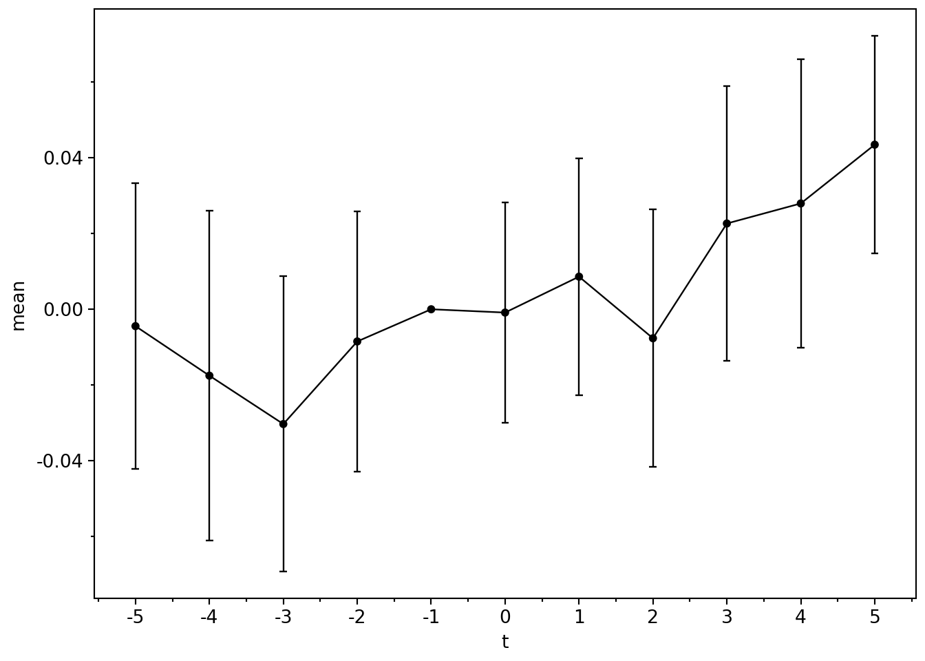
21.2.5 Discussion questions
The proprietary cost hypothesis tested by Li et al. (2018) posits that increased cost of disclosure will lead to reduced supply of disclosure. What rival theories exist that would make alternative predictions? Are there other elements of disclosure theory that might be tested? Why do you think Li et al. (2018) focused on this specific element of the proprietary cost hypothesis?
In the analysis above, we do not include the control variables considered by Li et al. (2018). For example, Li et al. (2018) “include R&D expenditures to sales, advertisement [sic] expenditure to sales, and intangible assets scaled by total assets to control for a firm’s proprietary costs of disclosure.” Using the approach outlined in Chapter 4, in what circumstances would it be necessary to control for “a firm’s proprietary costs of disclosure” in this way? Do these circumstances seem applicable in this setting, where the treatment is a (presumably exogenous) shock to disclosure costs and the outcome is disclosure choices?
What differs between the regressions reported in columns (1) and (3), and (2) and (4) of Table 21.4, respectively? Does this tell you anything about what drives the regression results in this setting? What happens if you omit the year fixed effects from both sets of regressions? What does this tell you about the role of the “non-switchers” (i.e., firms not in the
switchersdata frame) in the regression?Would you expect the inclusion of controls (see the question above) to have a significant impact on the regression results? Why or why not?
What differs between the regressions reported in columns (1) and (3), and (2) and (4) of Table 21.5, respectively? What happens if you omit the year fixed effects from both sets of regressions? What does this tell you about what drives the regression results in this setting?
What patterns do you observe in the coefficients reported in Table 21.5? Do these conform to what you would expect from Li et al. (2018)? (It may be easiest to focus on these in groups, e.g., those in \(t-5\) to \(t-2\), those in \(t + 0\) to \(t+3\) and those for \(t+4\) and \(t+5\).)
How do the variables in Table 21.5 differ from those used in Table 3 of Li et al. (2018)? Modify the code above (e.g.,
format_event_time()) to produce analysis closer to that reported in Table 3 of Li et al. (2018).The
format_event_time()function collapses years after \(t + 5\) and before \(t - 5\) into years \(t + 5\) and \(t - 5\), respectively. When would this approach make sense? What would be one alternative approach to handling these years? Does your suggested approach make a difference in this setting?How helpful do you find Figure 21.2 (plot of the coefficients by year)?
Describe the data set created from the following code. What proportion of the firms in the data set have
same_stateequal totrue? For the purposes of empirical analysis, do the firms withsame_stateequal tofalseenhance, or detract from, our ability to draw causal inferences about the effect of adoption of IDD?
switch_years_state = (
    reg_data_switchers
    .sort(["gvkey", "datadate"])
    .with_columns(
        pl.col("state", "period_type").shift(1).over("gvkey")
        .name.prefix("lag_")
    )
    .with_columns(
        same_state=pl.col("state") == pl.col("lag_state"),
        adoption_year=
            (pl.col("period_type") == "Post-adoption") &
            (pl.col("lag_period_type") == "Pre-adoption"),
    )
    .filter(pl.col("adoption_year"))
)- What issues might be implied by the following data? How might you address these?
(
    reg_data_t
    .group_by("t")
    .agg(pl.len().alias("n"))
    .sort("t")
    .style
    .fmt_integer()
)| t | n |
|---|---|
| −inf | 25,608 |
| −5 | 232 |
| −4 | 116 |
| −3 | 153 |
| −2 | 218 |
| −1 | 321 |
| 0 | 384 |
| 1 | 305 |
| 2 | 233 |
| 3 | 192 |
| 4 | 168 |
| 5 | 782 |
21.3 Further reading
Chapter 5 of Angrist and Pischke (2008) provides a good introduction to the topic of fixed effects and panel data. Chapters 8 and 9 of Cunningham (2021) go beyond the topics here and provide an excellent pathway to recent developments in the fixed-effects literature. Chapters 16 and 18 of Huntington-Klein (2021) also provide excellent coverage, including discussion of some issues not covered in this book.
Note that the function
get_test_scores()returns a version of the data that mergestest_scoresandcamp_attendanceand calculates thepostandtreatvariables we added in Chapter 3.↩︎This maximum exists not only because it seems inhumane to require even simulated students to attend school for longer but also because the grade effects are hard-coded and only for 12 years.↩︎
If you are curious, you can see this in the source code for the function: https://github.com/iangow/farr/blob/main/R/get_test_scores.R.↩︎
The parallel trends assumption is likely subtly violated because of regression-to-the mean effects in test scores, but not in a way likely to be detected using the usual “parallel trends plots” used in the literature. A researcher seeing the underlying data-generating process is likely to find it very easy to imagine the “can-opener” of parallel trends we discussed in Chapter 19. To paraphrase Macbeth: “Is this a [can-opener] which I see before me, The handle toward my hand? Come, let me clutch thee. I have thee not, and yet I see thee still. Art thou not, fatal vision, sensible To feeling as to sight? … Thou marshal’st me the way that I was going [i.e., to use DiD], And such an instrument I was to use.”↩︎
See Gartner (2011): https://go.unimelb.edu.au/yww8.↩︎
See the source code for the
farrpackage for details on the somewhat manual construction of this data set: https://github.com/iangow/farr/blob/main/data-raw/create_undisclosed_names.R. This likely mirrors a process used for Li et al. (2018) itself.↩︎See the source code for the
farrR package for the code used in creating this data set: https://github.com/iangow/farr/blob/main/data-raw/create_llz_2018_gvkeys.R.↩︎This data frame is derived from data provided by Bill McDonald. See Bill McDonald’s website for the original data: https://sraf.nd.edu/data/augmented-10-x-header-data/.↩︎
Any gaps are filled in by extending the
min_dateback to the date after the precedingmax_date.↩︎Note that
names_segprovides just one CIK for each GVKEY, though firms can change CIKs over time, which means that we will lose observations related to firms that previously used a different CIK from that found onnames_seg.↩︎Note that Li et al. (2018) include controls and more fixed effects, but these do not seem central to the analyses and we omit these↩︎