23  Beyond OLS

This part of the book explores some additional topics that are too advanced to be covered in Part I and that do not quite fit in Part III. These include generalized linear models (this chapter), extreme values and sensitivity analysis (Chapter 24), matching (Chapter 25), and a chapter on prediction that also introduces machine learning approaches (Chapter 26). Apart from Chapter 24 building on this chapter, the material in each of these chapters is largely independent of that in the others in this section. Material in this chapter and in Chapters 24 and 25 does build on ideas in Part III to some extent, but likely could be covered before Part III. The material in Chapter 26 is fairly discrete and could be tackled by students with the level of understanding provided by the first few chapters of Part I.

In Chapter 3, we studied the fundamentals of regression analysis with a focus on OLS regression. While we have used OLS as the foundation for almost all regression analyses so far, OLS will at times appear not to be appropriate. For example, if the dependent variable is binary, some aspects of OLS may be difficult to interpret and OLS may be econometrically inefficient. Examples of binary dependent variables include an indicator variable for accounting fraud (see Chapter 26) or for using a Big Four auditor (see Chapter 25).

Similar issues apply to inherently non-negative dependent variables, such as total assets or count variables, such as the number of management forecasts, the number of 8-K filings, or the number of press releases, as seen in Guay et al. (2016), the focus of this chapter.

In this chapter, we cover generalized linear models (GLMs), a class of models that includes probit and logit models—which assume a binary dependent variable—and Poisson regression—which is most naturally motivated by count variables.

A second theme of this chapter is the introduction of additional data skills relevant for applied researchers. In previous chapters we have eschewed larger data sets beyond those available through WRDS. However, most researchers need to know how to manage larger data sets, so we introduce some skills for doing so here.

In particular, we collect metadata for every filing made on the SEC EDGAR system since 1993, producing a data frame that occupies 3 GB if loaded into memory. While 3 GB certainly is not “big data”, it is large enough that more efficient ways of working have a significant impact on the facility of manipulating and analysing the data.

Tip

The code in this chapter uses the packages listed below. For instructions on how to set up your computer to use this code, go to the support page for this book. The support page also includes Quarto templates for the code and exercises below.

import os
from datetime import datetime

import numpy as np
import polars as pl
import polars.selectors as cs
import pyfixest as pf
from maketables import ETable

import statsmodels.api as sm
from scipy.stats import logistic, norm
import statsmodels.formula.api as smf

from era_pl import (
    ensure_lm_10x_summary_parquet,
    get_event_dates,
    sec_get_index,
    sec_index_available_update,
    sec_index_update,
    get_trading_dates,
    load_data,
    load_parquet,
    ptime,
    sec_index_update_all,
)
import plotnine_polars as p9
from plotnine_polars import aes

23.1 Complexity and voluntary disclosure

Like Li et al. (2018) (covered in Chapter 21), Guay et al. (2016) examine the phenomenon of voluntary disclosure. A core idea of Guay et al. (2016) is that users of a more complex firm’s disclosures require more information to understand the business sufficiently well to invest in it. Guay et al. (2016, p. 235) posit that “economic theory suggests that managers will use other disclosure channels to improve the information environment” when their reporting is more complex. A number of “other disclosure channels” are explored in Guay et al. (2016), including the issuance of management forecasts (the primary measure), filing of 8-Ks, and firm-initiated press releases.

Guay et al. (2016) find evidence of greater voluntary disclosure by firms with more complex financial statements. For example, Table 3 of Guay et al. (2016) presents results of OLS regressions with two different measures of financial statement complexity, and with and without firm fixed effects.

23.1.1 Discussion questions

1. Guay et al. (2016, p. 252) argue that the “collective results from our two quasi-natural experiments … validate that our text-based measures of financial statement complexity reflect, at least in part, the complexity of the underlying accounting rules.” Which specific table or figure of Guay et al. (2016) provides the most direct evidence in support of this claim? Can you suggest any alternative tests or presentations to support this claim?

2. What is the causal diagram implied by the regression specification in Table 3 of Guay et al. (2016)? Provide arguments for and against the inclusion of ROA, SpecialItems and Loss as controls.

3. Assuming that the causal effect of FS_complexity implied by the results in Table 3 exists, provide an explanation for the changes in the coefficients when firm fixed effects are added to the model. When might you expect these changes to have the opposite sign?

4. Guay et al. (2016, p. 234) conclude that “collectively, these findings suggest managers use voluntary disclosure to mitigate the negative effects of complex financial statements on the information environment.” Suppose you wanted to design a field experiment to test the propositions embedded in this sentence and were given the support of a regulator to do so (e.g., you can randomize firms to different regimes, as was done with Reg SHO discussed in Section 19.2). How would you implement this experiment? What empirical tests would you use? Are some elements of the hypothesis more difficult than others to test?

5. Clearly Guay et al. (2016) did not have the luxury of running a field experiment. Do you see any differences between the analyses you propose for your (hypothetical) field experiment and those in Guay et al. (2016)? What do you think best explains any differences?

23.2 Generalized linear models

In this section, we introduce the idea of generalized linear models (GLMs), which provides a powerful framework for analysing a wide class of settings beyond OLS. We begin by discussing maximum likelihood as an organizing principle for estimation before applying that to understand regression analysis with binary dependent variable.

After discussing the concept of marginal effects, we finish up this section with a discussion of GLM regressions with count variables.

23.2.1 Maximum likelihood

The concept of maximum likelihood estimation provides a useful framework for thinking about regression, including GLMs. As the name “ordinary least squares” suggests, OLS regression is often motivated as the linear estimator that minimizes the squared residuals in a setting in which \(y = X \beta\).

However, we can take another perspective. Suppose that \(y_i = X_i \beta + \epsilon_i\) where \(\epsilon_i \sim N(0, \sigma^2)\) and \(\epsilon_i\) is independent across individuals (\(i\)). As such, the density for \(y_i\) is given by

\[ f(y_i | X_i \beta) = \frac{1}{\sigma \sqrt{2 \pi}} \exp \left(-\frac{(y_i - X_i \beta)^2}{2\sigma^2} \right) \] But mathematically, the \(y_i\) and \(X_i\) can be seen as given and this function can be viewed instead as a function of \(\beta\) and relabelled as a likelihood function.

\[ \mathcal{L}(\beta; X_i, y_i) = \frac{1}{\sigma \sqrt{2 \pi}} \exp \left(-\frac{(y_i - X_i \beta)^2}{2\sigma^2} \right) \] Given independence, the density for the full sample \(y = (y_1, \dots, y_N)\) is simply the product of the densities of each observation and we can consider the likelihood function for the full sample in the same way.

\[ \mathcal{L}(\beta; X, y) = \prod_{i=1}^N \frac{1}{\sigma \sqrt{2 \pi}} \exp \left(-\frac{(y_i - X_i \beta)^2}{2\sigma^2} \right) \]

We can also write the log-likelihood as follows

\[ \begin{aligned} \log \mathcal{L}(\beta; X, y) &= \sum_{i=1}^N \left( \log \left(\frac{1}{\sigma \sqrt{2 \pi}} \right) + \left(-\frac{(y_i - X_i \beta)^2}{2\sigma^2} \right) \right) \\ &= \sum_{i=1}^N \log \left(\frac{1}{\sigma \sqrt{2 \pi}} \right) + \sum_{i=1}^N \left(-\frac{(y_i - X_i \beta)^2}{2\sigma^2} \right) \\ \end{aligned} \]

The idea of maximum likelihood estimation (MLE) is to choose the values \(\hat{\beta}\) and \(\hat{\sigma}\) that maximize the likelihood function. But note that maximizing the log-likelihood will yield the same solution as maximizing the likelihood (because \(\log(x) > \log(y) \Leftrightarrow x > y\)) and that only the second term in the sum above is affected by the value of \(\beta\).

This means that maximizing the log-likelihood with respect to \(\beta\) is achieved by maximizing the second term. But the second term is nothing but the negative of the sum of square residuals. So the least-squares estimator is the maximum likelihood estimator in this setting.

So why introduce MLE in the first place? First, this equivalence will not hold in general. Merely assuming heteroskedasticity (i.e., that \(\sigma_i^2 \neq \sigma_j^2\) for \(i \neq j\)) is enough to create a wedge between least-squares and MLE.

Second, MLE can be shown to have desirable econometric properties in a broad class of settings. According to Wooldridge (2010, p. 385), “MLE has some desirable efficiency properties: it is generally the most efficient estimation procedure in the class of estimators that use information on the distribution of the endogenous variables given the exogenous variables.” Additionally, MLE has “a central role” (Wooldridge, 2010, p. 386) in estimation of models with limited dependent variables, which we cover in the next section.

23.2.2 Binary dependent variables

If we have a setting in which \(y_i \in \{0, 1\}\) (i.e., the dependent variable is binary), then a generic framework has the conditional density of \(y_i\) as

\[ g(y_i | X_i; \beta ) = \begin{cases} h(X_i \cdot \beta), & y_i = 1 \\ 1 - h(X_i \cdot \beta), &y_i = 0 \\ 0, &\text{otherwise} \\ \end{cases} \]

where \(X = (1, x_{i1}, x_{i2}, \dots, x_{ik})\), \(\beta = (\beta_0, \beta_1, \dots, \beta_k)\), and \(h(\cdot)\) is a known function \(\mathbb{R} \to [0, 1]\).

With this setup, we define the logit model in terms of \(h(\cdot)\):

\[ h(X\beta) = \frac{e^{X\beta}}{1 + e^{X\beta}} \] The probit model is defined using the standard normal distribution function \(\Phi(\cdot)\):

\[ h(X\beta) = \Phi(X\beta) \] If we assume that one of the above functions describes the underlying data-generating process, then we can construct the corresponding maximum-likelihood estimator of \(\beta\). For example, the probit model implies that

\[ f_{Y|X} = g(Y, X; \beta) = \Phi(X \beta)^{Y} (1 - \Phi(X \beta))^{1- Y} \] \[ \mathcal{L}(\beta | Y, X) = \prod_{i = 1}^n \Phi(X_i \beta)^{Y_i} (1 - \Phi(X_i \beta))^{1- Y_i} \] \[ \begin{aligned} \log \mathcal{L}(\beta | Y, X) &= \log \left( \prod_{i = 1}^n \Phi(X_i \beta)^{Y_i} (1 - \Phi(X_i \beta))^{1- Y_i} \right) \\ &= \sum_{i = 1}^n \log \left( \Phi(X_i \beta)^{Y_i} (1 - \Phi(X_i \beta))^{1- Y_i} \right) \\ &= \sum_{i = 1}^n {Y_i} \log \Phi(X_i \beta) + (1 - Y_i) \log (1 - \Phi(X_i \beta)) \\ \end{aligned} \] Thus, given \(Y\) and \(X\), we can obtain the ML estimate of \(\beta\) using a computer to find

\[ \hat{\beta}_{ML} = \underset{\beta \in \mathbb{R^{k+1}}}{\arg \max} \sum_{i = 1}^n {Y_i} \log \Phi(X_i \beta) + (1 - Y_i) \log (1 - \Phi(X_i \beta)) \]

A similar analysis can be conducted for logit regression.

But rarely would a researcher have good reasons to believe strongly that the correct model is the probit model, rather than the logit model, or vice versa. This raises questions about the consequences of estimation using MLE, but with the wrong model. In other words, what happens if we use probit regression when the correct model is logit? Or logit regression when the correct model is probit? And what happens if we simply use OLS to fit a model? (The term linear probability model is used to describe the fitting of OLS with a binary dependent variable, as the fitted values can be interpreted as probabilities that \(y=1\), even though these fitted values can fall outside the \([0, 1]\) interval.)

A natural way to examine these questions is with simulated data. We make a small function (get_probit_data()) that generates data using the assumptions underlying the probit model. We generate random \(x\) and then calculate \(h(X\beta) = \Phi(X\beta)\), which gives us a vector h representing the probability that \(y_i = 1\) for each \(i\). We then compare \(h(X_i \beta)\) with \(u_i\), a draw from the uniform distribution over \([0, 1]\).¹ If \(h(X_i \beta) > u_i\), then \(y = 1\); otherwise \(y = 0\). If \(h(X_i \beta) = 0.9\) then we have a 90% chance that \(h(X_i \beta) > u_i\). Finally, the get_probit_data() function returns the generated data.

def get_probit_data(
    beta_0: float = -2.0,
    beta_1: float = 0.3,
    n: int = 1000,
    seed: int | None = None,
) -> pl.DataFrame:
    rng = np.random.default_rng(seed)
    x = rng.normal(size=n)
    h = norm.cdf(beta_0 + x * beta_1)
    y = rng.uniform(size=n) < h
    return pl.DataFrame({"x": x, "y": y.astype(np.int8)})

23.2.2.1 Marginal effects

An important concept with non-linear models such as those examined in this chapter is the marginal effect. Given a causal model \(\mathbb{E}[y|X] = f(X)\), the partial derivative of \(x_j\) at \(X = x\)—that is,

\[\left. \frac{\partial \mathbb{E}[y|X]}{\partial x_j} \right|_{X = x}\]

for \(j \in (1, \dots, k)\)—can be viewed as the marginal effect of a change in \(x_j\) on the value of \(\mathbb{E}[y|X]\) evaluated at \(X = x\).

If \(y\) is a binary variable, then \(\mathbb{E}[y_i|X_i] = \mathbb{P}[y_i = 1|X_i]\). If we have a probit model, then \(\mathbb{P}[y_i = 1|X_i] = \Phi(X_i \beta)\). Assuming that \(X_i\) is a continuous variable, we then have the following:²

\[ \begin{aligned} \frac{\partial \mathbb{E}[y_i|X_i]}{\partial x_{ij}} &= \frac{\partial \mathbb{P}[y_i = 1|X_i]}{\partial x_{ij}} \\ &= \frac{\partial \Phi(X_i \beta)}{\partial x_{ij}} \\ &= \frac{\partial \Phi(X_i \beta)}{\partial (X_i \beta)} \frac{\partial (X_i \beta)}{\partial x_{ij}} \\ &= \phi(X_i \beta) \beta_j \\ \end{aligned} \] That is, the marginal effect is the product of the probability density function and the coefficient \(\beta_j\). Note that we used the facts that the first derivative of the cumulative normal distribution \(\Phi(\cdot)\) is the normal density function \(\phi(\cdot)\) and that the partial derivative of \(X_i \beta = \beta_0 + x_{i1} \beta_1 + \dots + x_{ij} \beta_j + \dots + x_{ik} \beta_k\) with respect to \(x_{ij}\) is \(\beta_j\).

With linear models such as those fitted using OLS where \(x_j\) only enters the model in a linear fashion, the marginal effect of \(x_j\) is simply \(\beta_j\) and does not depend on the value \(x_j\) at which it is evaluated. But in models in which \(x_j\) interacts with other variables or enters the model in a non-linear fashion, the marginal effect of \(x_j\) can vary. For example, in the following model, the marginal effect of \(x_1\) will depend on the values of \(x_1\) and \(x_2\) at which it is evaluated.³

\[ y_i = \beta_0 + x_{i1} \beta_1 + x_{i2} \beta_2 + x_{i1} x_{i2} \beta_3 + x^2_{i2} \beta_4 + \epsilon_i \]

With non-linear models the marginal effect of \(x_j\) will generally depend on the value \(x\) at which it is evaluated. One common approach evaluates the marginal effect at the sample mean of \(\overline{X} = (\overline{x}_1, \dots, \overline{x}_k)\). Another approach would be to report the mean of the marginal effects evaluated for each \(X\) in the sample, but this approach may be difficult to interpret if the signs of the marginal effects vary across the sample distribution.

\[ \begin{aligned} \mathbb{E} \left[\frac{\partial \mathbb{E}[y_i|X_i]}{\partial x_{ij}} \right] &= \mathbb{E} \left[\phi(X_i \beta) \right] \beta_j \\ \end{aligned} \]

The following function implements the latter computation for probit, logit, and OLS models. While a more sophisticated version of this function would infer the model’s type from its attributes, this function is adequate for our needs here. The mfx package offers estimates of marginal effects for a variety of models.

def get_mfx(fm, model_type: str) -> float:
    X = fm.model.exog
    if model_type == "probit":
        pdf = float(norm.pdf(X @ fm.params).mean())
    elif model_type == "logit":
        pdf = float(logistic.pdf(X @ fm.params).mean())
    elif model_type == "Poisson":
        pdf = float(np.exp(X @ fm.params).mean())
    else:
        pdf = 1.0
    return float(pdf * fm.params[1])

The following fit_model() convenience function fits a model, extracts statistics from that model, then returns a data frame containing those statistics

def fit_model(data: pl.DataFrame, model_type: str = "OLS") -> pl.DataFrame:
    X = sm.add_constant(data["x"].to_numpy())
    y = data["y"].to_numpy()

    if model_type == "probit":
        fm = sm.Probit(y, X).fit(disp=0)
    elif model_type == "logit":
        fm = sm.Logit(y, X).fit(disp=0)
    elif model_type == "Poisson":
        fm = sm.Poisson(y, X).fit(disp=0)
    else:
        fm = sm.OLS(y, X).fit()

    return pl.DataFrame({
        "type": [model_type],
        "coef": [float(fm.params[1])],
        "se": [float(fm.bse[1])],
        "t_stat": [float(fm.tvalues[1])],
        "p": [float(fm.pvalues[1])],
        "mfx": [get_mfx(fm, model_type)],
    })

We then create a function to run an iteration of the simulation: it gets the data using get_probit_data(), extracts statistics using fit_model() for three different model types, then returns a data frame with the results.

def run_probit_sim(i: int, beta_1: float) -> pl.DataFrame:
    df = get_probit_data(beta_1=beta_1, seed=2024 + i)
    fits = [
        fit_model(df, model_type=t)
        for t in ("probit", "logit", "OLS")
    ]
    return (
        pl.concat(fits, how="vertical")
        .with_columns(
            i=pl.lit(i),
            beta_1_true=pl.lit(beta_1),
        )
        .select(
            "i", "beta_1_true", "type", "coef",
            "se", "t_stat", "p", "mfx"
        )
    )

Finally, we run the simulation n_iters times for each of two values of \(\beta_1\). We consider \(\beta_1 = 0\), so that the null hypothesis of no relation between \(x_1\) and \(y\) is true. We also consider \(\beta_1 = 0.3\), so that the null hypothesis of no relation between \(x_1\) and \(y\) is false. The former allows us to check that the rejection rate matches the size of the test (\(\alpha = 0.05\) or \(\alpha = 0.01\)). The latter provides insights into the power of the tests.

n_iters = 1000

with ptime():
    results = pl.concat(
        [
            run_probit_sim(i, beta_1)
            for beta_1 in (0.0, 0.3)
            for i in range(n_iters)
        ],
        how="vertical",
    )

Wall time: 4.237 s

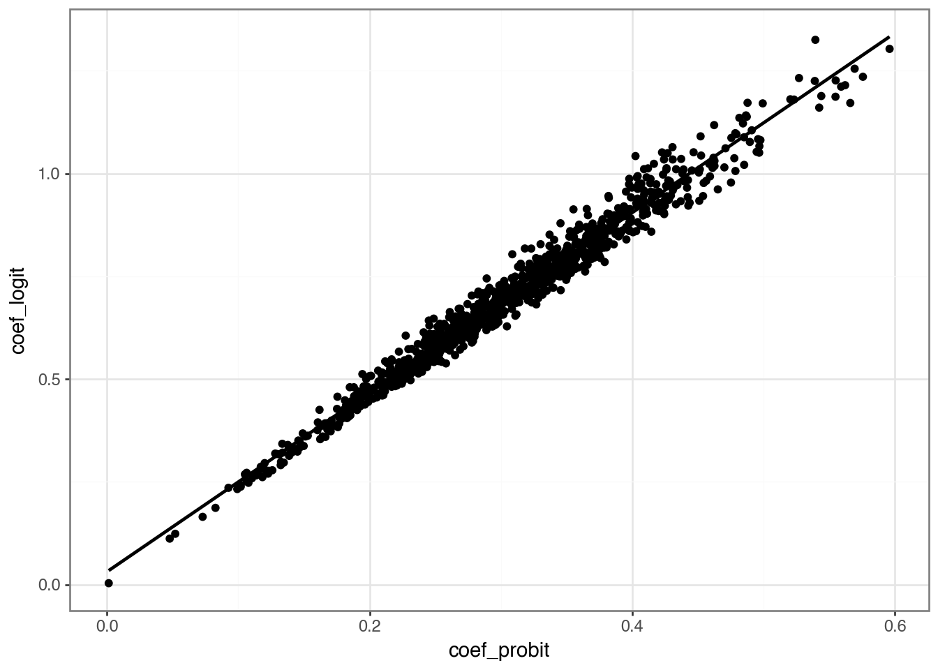
To understand the relationships between the various approaches, we focus on the case where \(\beta_1 \neq 0\) (so there is an underlying relationship between \(x\) and \(y\) to estimate).

rel_df = (
    results
    .filter(pl.col("beta_1_true") != 0)
    .pivot(index="i", on="type", values=["coef", "mfx"])
)

def fit_ols(formula, data):
    return smf.ols("coef_logit ~ coef_probit",
                   data=rel_df.to_pandas()).fit()

fms = [
    fit_ols("coef_logit ~ coef_probit", data=rel_df),
    fit_ols("coef_OLS ~ coef_probit", data=rel_df),
    fit_ols("mfx_logit ~ mfx_probit", data=rel_df),
    fit_ols("coef_OLS ~ mfx_probit", data=rel_df),
]

ETable(
    fms,
    model_heads=["Logit", "OLS", "mfx_logit", "mfx_OLS"],
    head_order="h",
    coef_fmt="b* \n (t)",
    signif_code=[0.01, 0.05, 0.10],
    model_stats=["N", "r2"],
    show_fe=False,
)

Table 23.1: Relationships between model coefficients

	Logit	OLS	mfx_logit	mfx_OLS
	(1)	(2)	(3)	(4)
coef
coef_probit	2.184*** (197.540)	2.184*** (197.540)	2.184*** (197.540)	2.184*** (197.540)
Intercept	0.031*** (8.839)	0.031*** (8.839)	0.031*** (8.839)	0.031*** (8.839)
stats
Observations	1,000	1,000	1,000	1,000
R2	0.975	0.975	0.975	0.975
Significance levels: * p < 0.1, ** p < 0.05, *** p < 0.01. Format of coefficient cell: Coefficient (t-stats)

(
    rel_df
    .ggplot(aes(x="coef_probit", y="coef_logit"))
    .geom_point()
    .geom_smooth(method="lm", se=False)
    .theme_bw()
)

Figure 23.1: Relationship between probit and logit model coefficients

(
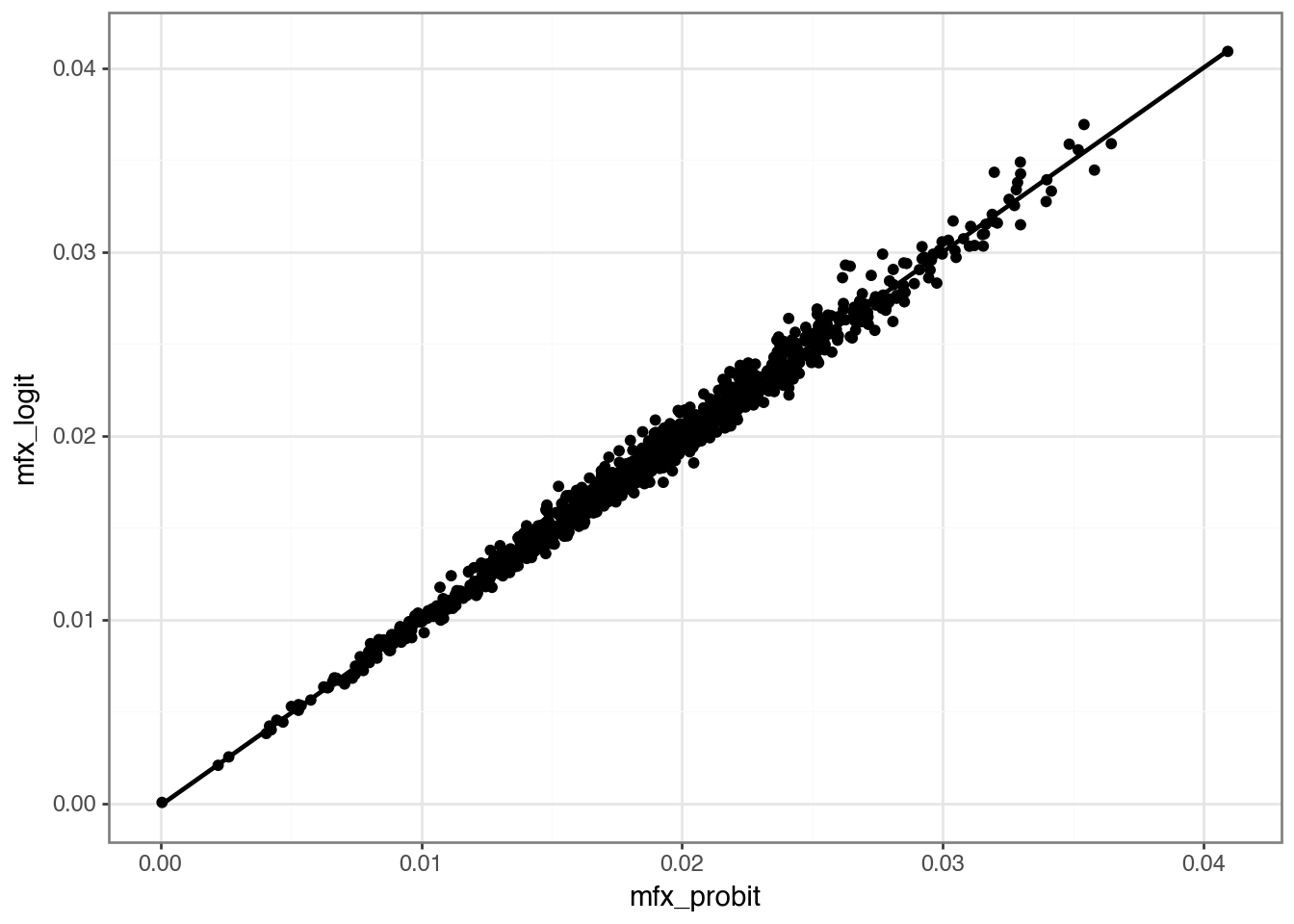
    rel_df
    .ggplot(aes(x="mfx_probit", y="mfx_logit"))
    .geom_point()
    .geom_smooth(method="lm", se=False)
    .theme_bw()
)

Figure 23.2: Relationship between probit and logit marginal effect estimates

(
    results
    .group_by("type", "beta_1_true")
    .agg(
        mean_coef=pl.col("coef").mean(),
        mean_mfx=pl.col("mfx").mean(),
        rej_rate_5=(pl.col("p") < 0.05).mean(),
        rej_rate_1=(pl.col("p") < 0.01).mean(),
    )
    .sort("beta_1_true", "type")
    .style
    .fmt_number(
        columns=["mean_coef", "mean_mfx",
                 "rej_rate_5", "rej_rate_1"],
        decimals=3,
    )
)

Table 23.2: Probit simulation results

type	beta_1_true	mean_coef	mean_mfx	rej_rate_5	rej_rate_1
OLS	0.0	0.000	0.000	0.052	0.014
logit	0.0	0.003	0.000	0.052	0.013
probit	0.0	0.001	0.000	0.051	0.012
OLS	0.3	0.018	0.018	0.940	0.831
logit	0.3	0.698	0.018	0.940	0.828
probit	0.3	0.305	0.018	0.939	0.820

23.2.3 Count variables

Another case in which OLS may be regarded as inadequate is when the dependent variable is a count variable. One member of the class of GLMs that models such a dependent variable is Poisson regression. In this model, we have \(y \sim \mathrm{Pois}(\mu)\) where \(\mu = \exp(\beta_0 + \beta_1 x)\).

def get_pois_data(
    beta_0: float = -2.0,
    beta_1: float = 0.3,
    n: int = 1000,
    seed: int | None = None,
) -> pl.DataFrame:
    rng = np.random.default_rng(seed)
    x = rng.normal(size=n)
    h = np.exp(beta_0 + x * beta_1)
    y = rng.poisson(lam=h)
    return pl.DataFrame({"x": x, "y": y})

def run_pois_sim(i: int, beta_1: float) -> pl.DataFrame:
    df = get_pois_data(beta_1=beta_1, seed=2024 + i)
    fits = [fit_model(df, model_type=t) for t in ("Poisson", "OLS")]
    return (
        pl.concat(fits, how="vertical")
        .with_columns(
            i=pl.lit(i),
            beta_1_true=pl.lit(beta_1),
        )
        .select(
            "i", "beta_1_true", "type", "coef",
            "se", "t_stat", "p", "mfx"
        )
    )

with ptime():
    results_pois = pl.concat(
        [
            run_pois_sim(i, beta_1)
            for beta_1 in (0.0, 0.3)
            for i in range(n_iters)
        ],
        how="vertical",
    )

Wall time: 1.873 s

(
    results_pois
    .group_by("type", "beta_1_true")
    .agg(
        mean_coef=pl.col("coef").mean(),
        mean_mfx=pl.col("mfx").mean(),
        rej_rate_5=(pl.col("p") < 0.05).mean(),
        rej_rate_1=(pl.col("p") < 0.01).mean(),
    )
    .sort("beta_1_true", "type")
    .style
    .fmt_number(
        columns=["mean_coef", "mean_mfx",
                 "rej_rate_5", "rej_rate_1"],
        decimals=3,
    )
)

Table 23.3: Poisson simulation results

type	beta_1_true	mean_coef	mean_mfx	rej_rate_5	rej_rate_1
OLS	0.0	−0.001	−0.001	0.040	0.012
Poisson	0.0	−0.004	−0.001	0.040	0.012
OLS	0.3	0.042	0.042	0.942	0.826
Poisson	0.3	0.299	0.042	0.942	0.830

23.3 Application: Complexity and voluntary disclosure

To enrich our understanding of GLMs and to examine some additional data skills, we return to a setting similar to that considered in Guay et al. (2016). Like Guay et al. (2016), we examine the association between complexity of financial reporting and subsequent voluntary disclosures. Our purpose here is not to conduct a close replication of Guay et al. (2016). In place of the measures used there, we use measures that are readily available.

This is the first chapter in which we need to collect a substantial amount of data from sources other than WRDS. To facilitate this, we perform a number of data steps as fairly discrete steps. This allows us to rerun code for one data set without requiring us to rerun code for other data sets.

We use parquet files for persistent storage. The helper function save_parquet() (defined above) takes either a lazy or eager Polars object and writes it to a schema subdirectory under DATA_DIR.

23.3.1 Measures of reporting complexity

Guay et al. (2016) consider a number of measures of reporting complexity, including readability and length. Loughran and McDonald (2014) argue that 10-K document file size provides a simple and useful proxy, so we use that here.

Data on 10-K document file size can be collected from SEC EDGAR, but gathering these directly would involve costly web scraping. So we use the Loughran-McDonald 10X summaries CSV and convert it to parquet.

ensure_lm_10x_summary_parquet()

PosixPath('/Users/igow/Dropbox/pq_data/glms/lm_10x_summary.parquet')

(
    load_parquet("lm_10x_summary", "glms")
    .with_columns(year=pl.col("filing_date").dt.year())
    .group_by("year")
    .agg(pl.len().alias("n"))
    .sort("year")
    .collect()
)

shape: (29, 2)

year	n
i32	u32
1993	13
1994	9752
1995	21880
1996	44531
1997	55484
…	…
2017	28755
2018	28017
2019	27014
2020	26184
2021	29320

23.3.2 Data on EDGAR filings

We also use SEC EDGAR index files. For each quarter, EDGAR provides a company.gz file with fixed-width records.

Because SEC does not allow anonymous downloads, our requests include a user-agent header via the USER_AGENT environment variable. If you have not set this in the .env file in the folder you are using to run the code, you can set it directly:

os.environ["USER_AGENT"] = "your_name@email.org"

The function sec_get_index() from the era_pl package processes the index file for a single quarter and saves it as a Parquet file under the edgar subdirectory of DATA_DIR.

with ptime():
    sec_index_2022q2 = sec_get_index(2022, 2, overwrite=True)

Wall time: 1.719 s

(
    sec_index_2022q2
    .select("company_name", "cik", "form_type", "date_filed", "file_name")
    .show()
)

shape: (5, 5)

company_name	cik	form_type	date_filed	file_name
str	i32	str	date	str
"006 - Series of IPOSharks Vent…	1894348	"D"	2022-04-08	"edgar/data/1894348/0001892986-…
"008 - Series of IPOSharks Vent…	1907507	"D"	2022-06-07	"edgar/data/1907507/0001897878-…
"01 Advisors 03, L.P."	1921173	"D"	2022-05-20	"edgar/data/1921173/0001921173-…
"01Fintech LP"	1928541	"D"	2022-05-13	"edgar/data/1928541/0001928541-…
"07 Carbon Capture, LP"	1921663	"D"	2022-04-05	"edgar/data/1921663/0001921663-…

Because SEC index files are continually being updated, we might want to update our local repository without redownloading files unnecessarily. The sec_index_available_update() function scrapes and returns the “last modified” information for a given year and quarter from the SEC website.

sec_index_available_update(2022, 2).strftime("%Y-%m-%d %H:%M:%S %Z")

'2022-06-30 22:22:05 EDT'

This information can be compared with information stored in the metadata of the Parquet file created by sec_get_index() above. This function allows sec_index_update() to only update a file if there’s an newer file on the SEC website.

sec_index_update(2022, 2)

2022 Q2: Index file is up to date.

False

The sec_index_update_all() function runs sec_index_update() for all quarters between 1993 Q1 (the first available on SEC EDGAR) and the current quarter.

with ptime():
    index_files_downloaded = sec_index_update_all()

Wall time: 62.290 s

After running the code above, we have 134 SEC index parquet files occupying about 497 MB of drive space.

We can load these files using load_parquet() and a wild card or glob pattern (*).

sec_index = load_parquet("sec_index_*", "edgar")
(
    sec_index
    .select("company_name", "cik", "form_type", "date_filed", "file_name")
    .show()
)

shape: (5, 5)

company_name	cik	form_type	date_filed	file_name
str	i32	str	date	str
"MERRILL LYNCH LIFE VARIABLE AN…	880794	"NSAR-B"	1993-02-26	"edgar/data/880794/9999999997-0…
"RBS PARTNERS L P /CT"	860585	"13FCONP"	1993-02-11	"edgar/data/860585/9999999997-0…
"SMITH THOMAS W"	926688	"13F-HR"	1993-02-12	"edgar/data/926688/9999999997-0…
"STORAGE TECHNOLOGY CORP"	94673	"CERTNYS"	1993-02-24	"edgar/data/94673/9999999997-05…
"MERRILL LYNCH LIFE VARIABLE AN…	880794	"POS AMI"	1993-04-28	"edgar/data/880794/9999999997-0…

(
    sec_index
    .with_columns(
        year=pl.col("date_filed").dt.year(),
        quarter=pl.col("date_filed").dt.quarter(),
    )
    .group_by("year", "quarter")
    .agg(pl.len().alias("n"))
    .sort("year", "quarter")
    .collect()
)

shape: (134, 3)

year	quarter	n
i32	i8	u32
1993	1	4
1993	2	4
1993	3	7
1993	4	20
1994	1	20879
…	…	…
2025	2	331536
2025	3	286771
2025	4	275728
2026	1	368379
2026	2	170247

(
    sec_index
    .group_by("form_type")
    .agg(pl.len().alias("n"))
    .sort("n", descending=True)
    .show(10)
)

Table 23.4: Most common form types on SEC EDGAR

shape: (10, 2)

form_type	n
str	u32
"4"	9546970
"8-K"	2065732
"424B2"	1026125
"SC 13G/A"	867478
"3"	866155
"10-Q"	711163
"6-K"	568649
"497"	535131
"D"	470005
"SC 13G"	456345

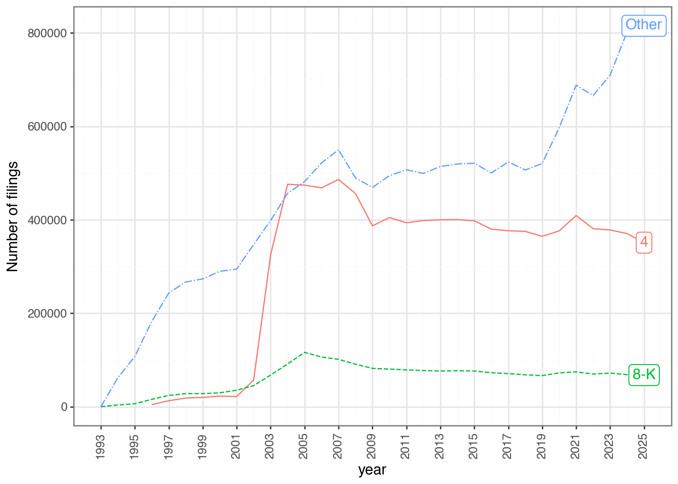
current_year = datetime.now().year
(
    sec_index
    .with_columns(
        year=pl.col("date_filed").dt.year(),
        form_type=pl.when(pl.col("form_type").is_in(["4", "8-K"]))
        .then(pl.col("form_type"))
        .otherwise(pl.lit("Other")),
    )
    .filter(pl.col("year") < pl.col("year").max())
    .group_by("year", "form_type")
    .agg(pl.len().alias("n"))
    .with_columns(
        last_year=pl.col("year") == pl.col("year").max()
    )
    .with_columns(
        label=pl.when(pl.col("last_year"))
                .then(pl.col("form_type"))
    )
    .sort("year", "form_type")
    .collect()
    .ggplot(aes(x="year", y="n", 
                color="form_type", linetype="form_type"))
    .geom_line()
    .geom_label(aes(label = "label"), na_rm = True)
    .scale_y_continuous(name="Number of filings")
    .scale_x_continuous(breaks=list(range(1993, current_year + 1, 2)))
    .theme_bw()
    .add_theme(axis_text_x=p9.element_text(angle=90), 
               legend_position="none")
)

Figure 23.3: Number of filings over time by type

(
    sec_index
    .filter(pl.col("form_type").str.contains(r"^8-K"))
    .group_by("form_type")
    .agg(pl.len().alias("n"))
    .with_columns(pl.col("n").truediv(pl.col("n").sum())
                  .mul(100).alias("percent"))
    .sort("n", descending=True)
    .collect()
    .style
    .fmt_integer(columns="n")
    .fmt_number(columns="percent", decimals=2)
)

Table 23.5: Number of 8-K filings by variant

form_type	n	percent
8-K	2,065,732	95.95
8-K/A	85,842	3.99
8-K12G3	652	0.03
8-K12B	361	0.02
8-K12G3/A	116	0.01
8-K15D5	78	0.00
8-K12B/A	42	0.00
8-K15D5/A	4	0.00

23.3.3 Measure of financial statement complexity

Our basic unit of observation is a 10-K filing. We retain acc_num, cik, the filing and reporting-period dates, and grossfilesize, then link filings to gvkey and iid using the gvkey_ciks table provided by era_pl.

lm_10x_summary = load_parquet("lm_10x_summary", "glms")
gvkey_ciks = load_data("gvkey_ciks").lazy()

filing_10k_merged = (
    lm_10x_summary
    .filter(pl.col("form_type") == "10-K")
    .join(gvkey_ciks, on="cik", how="inner")
    .filter(pl.col("filing_date")
            .is_between(pl.col("first_date"), 
                        pl.col("last_date")))
    .select("gvkey", "iid", "acc_num", "cik",
            "filing_date", "cpr", "grossfilesize")
    .with_columns(eomonth=pl.col("cpr").dt.month_end())
)

23.3.4 Measure of voluntary disclosure

We construct a measure of voluntary disclosure based on 8-K filings around the filing date of the 10-K. We keep all 8-K filings between one year before and one year after the 10-K filing date and then count filings in several windows.

filing_8k = (
    sec_index
    .filter(pl.col("form_type") == "8-K")
    .select(
        "cik",
        pl.col("date_filed").alias("date_8k"),
    )
)

vdis_df = (
    filing_10k_merged
    .rename({"filing_date": "fdate"})
    .with_columns(
        fdate_p1=pl.col("fdate").dt.offset_by("1y"),
        fdate_m1=pl.col("fdate").dt.offset_by("-1y"),
    )
    .join_where(
        filing_8k,
        pl.col("cik") == pl.col("cik_right"),
        pl.col("date_8k").is_between(
            pl.col("fdate_m1"), pl.col("fdate_p1")
        ),
    )
    .drop("cik_right")
    .with_columns(
        datediff=(pl.col("date_8k") - pl.col("fdate")).dt.total_days()
    )
    .group_by("acc_num", "gvkey", "iid", "cik")
    .agg(
        vdis_p1y=(pl.col("datediff") > 0).sum(),
        vdis_p30=pl.col("datediff").is_between(0, 30).sum(),
        vdis_p60=pl.col("datediff").is_between(0, 60).sum(),
        vdis_p90=pl.col("datediff").is_between(0, 90).sum(),
        vdis_m1y=(pl.col("datediff") < 0).sum(),
        vdis_m30=pl.col("datediff").is_between(-30, -1).sum(),
        vdis_m60=pl.col("datediff").is_between(-60, -1).sum(),
        vdis_m90=pl.col("datediff").is_between(-90, -1).sum(),
    )
)

23.3.5 Controls

In addition to our measure of voluntary disclosure (vdis_df) and our measure of financial statement complexity (filing_10k_merged), we need controls based on Compustat and CRSP. In the Python version we derive these directly from local parquet files rather than persisting them as intermediate parquet outputs.

23.3.5.1 Fundamental data from comp.funda

compustat = (
    load_parquet("funda", "comp")
    .filter(
        pl.col("indfmt") == "INDL",
        pl.col("datafmt") == "STD",
        pl.col("popsrc") == "D",
        pl.col("consol") == "C"
    )
    .with_columns(
        mkt_cap=pl.col("prcc_f") * pl.col("csho"),
    )
    .with_columns(
        size=pl.col("mkt_cap").log(),
        roa=pl.col("ib").era.div_if_pos("at"),
        mtb=pl.col("mkt_cap").era.div_if_pos("ceq"),
        special_items=(
            pl.col("spi").fill_null(0).era.div_if_pos("at")
        ),
        fas133=pl.col("aocidergl") != 0,
        fas157=pl.col("tfva") != 0,
    )
    .filter(pl.col("mkt_cap") > 0)
    .select(
        "gvkey", "iid", "datadate", "mkt_cap", "size",
        "roa", "mtb", "special_items", "fas133", "fas157"
    )
    .with_columns(eomonth=pl.col("datadate").dt.month_end())
)

23.3.5.2 Data on event dates for GVKEYs

ccm_link = (
    load_parquet("ccmxpf_lnkhist", "crsp")
    .filter(
        pl.col("linktype").is_in(["LC", "LU", "LS"]),
        pl.col("linkprim").is_in(["C", "P"])
    )
    .with_columns(linkenddt=pl.col("linkenddt")
                  .fill_null(pl.col("linkenddt").max()))
    .rename({"lpermno": "permno", "liid": "iid"})
)

filing_permnos = (
    filing_10k_merged
    .join(ccm_link, on=["gvkey", "iid"], how="inner")
    .filter(pl.col("filing_date")
            .is_between(pl.col("linkdt"), 
                        pl.col("linkenddt")))
    .select("gvkey", "iid", "filing_date", "permno")
    .unique()
)

event_dates = (
    get_event_dates(
        data=filing_permnos.select(
            pl.col("permno"),
            pl.col("filing_date").alias("event_date"),
        ).unique(),
        permno="permno",
        event_date="event_date",
        win_start=-20,
        win_end=20,
    )
    .rename({"event_date": "filing_date"})
    .join(filing_permnos, 
          on=["permno", "filing_date"], how="inner")
)

23.3.5.3 Data on “trading dates”

We first saw the trading_dates table in Chapter 12. Here we derive it directly from local crsp.dsi parquet data.

trading_dates = (
    get_trading_dates(load_parquet("dsi", "crsp"))
    .sort("date")
)

23.3.5.4 Data on liquidity measures

A core idea of Guay et al. (2016) is that firms use voluntary disclosure to mitigate the deleterious effects of financial statement complexity. One of the costs of greater financial statement complexity is greater illiquidity in the market for a firm’s equity. Guay et al. (2016) examine two primary measures of liquidity: the Amihud measure and the bid-ask spread.

first_year, last_year = (
    filing_10k_merged
    .select(
        first_year = pl.col("filing_date").dt.year().min() - 1,
        last_year = pl.col("filing_date").dt.year().max() + 1,
    )
    .collect()
    .row(0)
)

liquidity = (
    load_parquet("dsf", "crsp")
    .filter(
        pl.col("date").dt.year().is_between(
            first_year, last_year
        )
    )
    .with_columns(cs.decimal().cast(pl.Float64))
    .with_columns(
        pl.col("prc").abs(),
        (pl.col("vol") * pl.col("prc").abs()).alias("vol_val"),
    )
    .with_columns(
        spread=(
            (pl.col("ask") - pl.col("bid"))
            .era.div_if_pos("prc")
        ),
        illiq=(
            pl.col("ret").abs()
            .era.div_if_pos("vol_val")
        ),
    )
    .with_columns(
        spread=pl.col("spread") * 100,
        illiq=pl.col("illiq") * 1e6,
    )
    .filter(pl.all_horizontal(
        pl.col("spread", "illiq").is_not_null()))
    .select("permno", "date", "spread", "illiq")
)

23.3.6 Empirical analysis

Now that we have collected the data we need, we can run the final analysis. We begin by combining event dates with liquidity data. We then use trading_dates to map each filing date and each observation date to trading-day indices.

liquidity_merged = (
    event_dates
    .join_where(
        liquidity,
        pl.col("permno") == pl.col("permno_right"),
        pl.col("date").is_between(pl.col("start_date"), 
                                  pl.col("end_date")),
    )
    .drop("permno_right")
    .join(
        trading_dates.rename(
            {"date": "filing_date", "td": "filing_td"}
        ),
        on="filing_date",
        how="inner",
    )
    .join(trading_dates, on="date", how="inner")
    .with_columns(rel_td=pl.col("td") - pl.col("filing_td"))
    .select(
        "gvkey", "iid", "permno", "filing_date",
        "rel_td", "spread", "illiq"
    )
)

Some analyses in Guay et al. (2016) reduce complexity measures to either quintiles or deciles and we use quintiles for the complexity measure here. To allow for secular changes in complexity over time, we form quintiles by the year of filing_date.

complexity = (
    filing_10k_merged
    .with_columns(year=pl.col("filing_date").dt.year())
    .with_columns(
        complex_q5=pl.col("grossfilesize")
                   .era.ntile(5).over("year")
    )
)

Like Guay et al. (2016), we impose a sample requirement of complete data in the 20 trading days prior to the filing of the 10-K.

complete_cases = (
    liquidity_merged
    .filter(pl.col("rel_td") < 0)
    .group_by("gvkey", "iid", "filing_date")
    .agg(pl.len().alias("num_obs"))
    .filter(pl.col("num_obs") == 20)
    .select("gvkey", "iid", "filing_date")
)

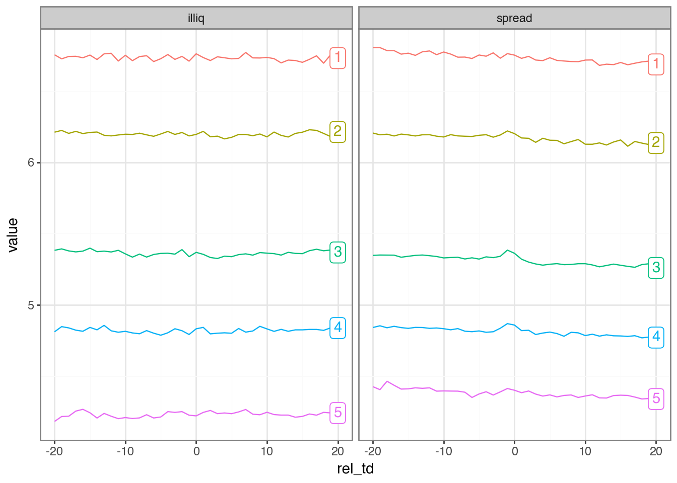
To better understand the underlying relations in the data, we examine the behaviour of measures of illiquidity around event dates by complexity quintile. We form deciles by year for the two measures of illiquidity.

with ptime():
    plot_data = (
        complexity
        .join(
            liquidity_merged,
            on=["gvkey", "iid", "filing_date"],
            how="inner",
        )
        .join(complete_cases, 
              on=["gvkey", "iid", "filing_date"], 
              how="inner")
        .with_columns(
            pl.col("spread", "illiq")
            .era.ntile(10)
            .over("year")
            .name.suffix("_decile")
        )
        .group_by("rel_td", "complex_q5")
        .agg(
            pl.col("spread_decile", "illiq_decile")
            .mean()
            .name.replace("_decile", ""),
            pl.len().alias("num_obs"),
        )
        .unpivot(
            index=["rel_td", "complex_q5", "num_obs"],
            on=["spread", "illiq"],
            variable_name="measure",
            value_name="value",
        )
        .with_columns(pl.col("complex_q5").cast(pl.String))
        .collect()
    )

Wall time: 17.439 s

labels_df = (
    plot_data
    .sort("rel_td")
    .group_by("measure", "complex_q5")
    .agg(
        pl.col("rel_td").last(),
        pl.col("value").last(),
        pl.col("num_obs").last(),
    )
)

(
    plot_data
    .ggplot(aes(x="rel_td", y="value", 
                color="complex_q5", group="complex_q5"))
    .geom_line()
    .geom_label(
        data=labels_df,
        mapping=aes(label="complex_q5"),
        show_legend=False,
    )
    .facet_wrap("~ measure")
    .theme_bw()
    .add_theme(legend_position="none")
)

Figure 23.4: Behaviour of illiquidity around 10-K filing dates by complexity quintile

To conduct regression analysis analogous to that in Table 3 of Guay et al. (2016), we combine our data on voluntary disclosure (vdis_df) with our data on financial statement complexity (filing_10k_merged) and controls (compustat).

reg_data_glms = (
    vdis_df
    .join(
        filing_10k_merged,
        on=["acc_num", "gvkey", "iid", "cik"],
        how="inner",
    )
    .join(compustat, on=["gvkey", "iid", "eomonth"], how="inner")
    .with_columns(pl.col("grossfilesize").log().name.prefix("ln_"))
    .collect()
)

We run three regressions. The first two are, following Guay et al. (2016), OLS with and without firm fixed effects. The third regression is Poisson regression.

controls = ["mkt_cap", "size", "roa", "mtb", "special_items"]
model = "vdis_p1y ~ " + " + ".join(["ln_grossfilesize", *controls])

fm_ols = pf.feols(model, data=reg_data_glms)
fm_fe = pf.feols(model + " | gvkey + iid", data=reg_data_glms)
fm_pois = (
    sm.GLM.from_formula(model, data=reg_data_glms.to_pandas(), 
                        family=sm.families.Poisson())
    .fit(cov_type="HC1")
)

We use “robust” standard errors for the Poisson regression as, based on papers we examine in Chapter 24, this seems to be a standard practice with Poisson regression.

ETable(
    [fm_ols, fm_fe, fm_pois],
    model_heads=["OLS", "Firm FE", "Poisson"],
    head_order="h",
    coef_fmt="b:.3f* \n (se:.3f)",
    signif_code=[0.01, 0.05, 0.10],
    model_stats=["N"],
)

Table 23.6: Financial statement complexity and voluntary disclosure

	OLS	Firm FE	Poisson
	(1)	(2)	(3)
coef
ln_grossfilesize	1.790*** (0.013)	1.391*** (0.015)	0.187*** (0.001)
mkt_cap	-0.000 (0.000)	0.000 (0.000)	-0.000*** (0.000)
size	0.532*** (0.010)	0.433*** (0.022)	0.054*** (0.001)
roa	-0.003 (0.004)	-0.028** (0.012)	-0.000 (0.000)
mtb	-0.000* (0.000)	-0.000 (0.000)	-0.000 (0.000)
special_items	0.004 (0.004)	0.023** (0.010)	0.000 (0.000)
Intercept	-19.708*** (0.184)		-0.853*** (0.020)
fe
iid	-	x	-
gvkey	-	x	-
stats
Observations	105,521	103,115	105,521
Significance levels: * p < 0.1, ** p < 0.05, *** p < 0.01. Format of coefficient cell: Coefficient (Std. Error)

23.3.7 Exercises

1. What benefits do you see from converting the external inputs to parquet once rather than reparsing the raw files each time?

2. What primary key could we use for lm_10x_summary? Check that this is a valid primary key.

3. What primary key could we use for filing_10k_merged? Check that this is a valid primary key.

4. From Figure 23.4, do you observe a change in measures of liquidity around 10-K filing dates? Why or why not would we expect to see a change around these events?

5. From Figure 23.4, do you observe a relation between the complexity of financial statements and illiquidity? Is the sign of any relationship consistent with what we would expect from reading Guay et al. (2016)?

6. Calculate the marginal effects associated with the regression coefficients shown in Table 23.6. Do you observe significant differences across specifications? (Hint: The marginal effect for the linear models is just the relevant coefficient; for the Poisson model, use the fitted conditional mean.)

23.4 Further reading

Chapter 13 of Wooldridge (2010) provides a more thorough discussion of MLE. Chapter 15 of Wooldridge (2010) covers probit and logit, including MLE and marginal effects. Chapter 19 of Wooldridge (2010) covers count models, including Poisson regression. We demonstrated that OLS works well for practical purposes with simulated data, and Angrist and Pischke (2008) likewise highlight cases where it delivers very similar inferences.

For more on GLMs, including details about estimation of coefficients and standard errors, see Dunn and Smyth (2018). Aronow and Miller (2019) provide a modern take on MLE estimation.

Angrist, J.D., Pischke, J.-S., 2008. Mostly harmless econometrics: An empiricist’s companion. Princeton University Press.

Aronow, P.M., Miller, B.T., 2019. Foundations of agnostic statistics. Cambridge University Press. https://doi.org/10.1017/9781316831762

Dunn, P.K., Smyth, G.K., 2018. Generalized linear models with examples in R, Springer Texts in Statistics. Springer New York. https://doi.org/10.1007/978-1-4419-0118-7

Guay, W.R., Samuels, D., Taylor, D.J., 2016. Guiding through the fog: Financial statement complexity and voluntary disclosure. Journal of Accounting and Economics 62, 234–269. https://doi.org/10.1016/j.jacceco.2016.09.001

Li, Y., Lin, Y., Zhang, L., 2018. Trade secrets law and corporate disclosure: Causal evidence on the proprietary cost hypothesis. Journal of Accounting Research 56, 265–308. https://doi.org/10.1111/1475-679X.12187

Loughran, T., McDonald, B., 2014. Measuring readability in financial disclosures. The Journal of Finance 69, 1643–1671. https://doi.org/10.1111/jofi.12162

Wooldridge, J.M., 2010. Econometric analysis of cross section and panel data, 2nd ed. MIT Press.

---

1. Some sources will formulate the data-generating process in a different, but equivalent, fashion. For example, Angrist and Pischke (2008) posit a latent variable \(y^{*}_i = X_i \beta - \nu_i\), where \(\nu_i \sim N(0, \sigma^2_{\nu})\).

2. Note that we have suppressed the evaluation of these quantities at \(X=x\) for reasons of space and clarity.

3. Note that this is still a linear model because it is linear in its coefficients.