2 Get Started

I don’t disagree with anything that Healy (2026) says in Chapter 2.

In the current version of this guide, I assume that you are already familiar with Python. If you are unfamiliar with Python and just want to learn a bit about data visualization, I would recommend just using R and Healy (2026). Even if your ultimate destination is Python, whatever you learn from R will largely carry over to Python. Getting started with data analysis is simply easier with R and, if you are not destined to learn Python, it’s probably a better path for many users.

For example, the Python ecosystem is built around things like virtual environments and, even with tools like uv, these are not easy for newcomers to manage, especially when using Jupyter notebooks. In contrast, I would get that most R users have a single system-level installation of the packages they use and virtual environments are reserved for special use cases.

In writing this guide, I have made a couple of additional choices that may make it not for you.

I use Python Polars: I have elected to use Python Polars as my data frame library rather than the more conventional choice of pandas. This choice partly reflects my choice of Polars in other settings (e.g., Polars is clearly the better choice for the larger data sets used in the book Empirical Research in Accounting). Another reason to use Polars is the second choice.
I use a “fluent” implementation of plotnine: While Healy (2026) uses ggplot2 package in R, the closest equivalent in Python is plotnine. However the plotnine package mimics ggplot2 so closely that it feels a bit like writing R code in Python. For a more “Pythonic” feel, I create a small package plotnine_polars, that provides a version of plotnine that creates a custom Polars data frame namespace that provides a “fluent” API for plotnine. It seems that “fluent” is a term of art in Python used to descibe APIs that implement functions as chainable methods.

2.1 Work in Plain Text

Everything Healy (2026) says here carries over to Python. I would recommend Quarto for Python too. While many Python users are more accustomed to using Jupyter notebooks (as they are now called), I believe that Quarto documents do a better job of separating source code from output.¹ This is particularly important when using source control systems such as Git.

The same “three backticks” approach discussed by Healy for R applies with Python too. Just use {python} in place of {r}:

```{python}

```

2.2 Use Python with an IDE

I writing this I am using Positron. This is probably a good choice for this project because it comes with Quarto.

At some point, I will put better instructions here.

2.3 Things to know about Python

While I assume that the following will be familiar, I think it is helpful to mirror a few observations from Healy (2026).

2.3.1 Everything has a name

True for Python too.

2.3.2 Everything is an object

Also true in Python. In many ways, Python is more object-oriented than R is, with many packages implementing functionality as methods that would be functions in R.

2.3.3 You do things using functions

If one recognizes that methods are simply functions attached to objects, this is also true of Python. If you’re coming from Stata or SAS, you may be used to thinking of functions (or “macros”) as a relatively advanced topic, both the R version and the Python version of Empirical Research in Accounting start with functions.

2.3.4 Functions come in packages

This is even more true in Python than it is in R. While R offers tools for working with arrays and data frames out of the box, Python relies much more on third-party packages for standard data science work. For example, arrays typically come from NumPy and data frames from packages such as pandas or Polars.

In this chapter, I use the following two packages.

import polars as pl
import plotnine_polars as p9
from plotnine_polars import aes
from socviz_pl import theme_socviz

p9.theme_set(theme_socviz())

These lines do not make any functions part of the namespace directly; one still needs to access them using (say) pl.read_csv(). In contrast, the command library(ggplot2) in R is closer to saying from polars import *; if we took that approach, read_csv() would become available directly.

2.3.5 “Ask vectors their type; ask complex objects their class”

It is difficult to do a literal translation of this to Python. To make things concrete let’s create an object.

gapminder = pl.read_csv(
    "https://raw.githubusercontent.com/jennybc/"
    "gapminder/main/inst/extdata/gapminder.tsv",
    separator="\t"
)
gapminder

shape: (1_704, 6)

country	continent	year	lifeExp	pop	gdpPercap
str	str	i64	f64	i64	f64
"Afghanistan"	"Asia"	1952	28.801	8425333	779.445314
"Afghanistan"	"Asia"	1957	30.332	9240934	820.85303
"Afghanistan"	"Asia"	1962	31.997	10267083	853.10071
"Afghanistan"	"Asia"	1967	34.02	11537966	836.197138
"Afghanistan"	"Asia"	1972	36.088	13079460	739.981106
…	…	…	…	…	…
"Zimbabwe"	"Africa"	1987	62.351	9216418	706.157306
"Zimbabwe"	"Africa"	1992	60.377	10704340	693.420786
"Zimbabwe"	"Africa"	1997	46.809	11404948	792.44996
"Zimbabwe"	"Africa"	2002	39.989	11926563	672.038623
"Zimbabwe"	"Africa"	2007	43.487	12311143	469.709298

Here we can see that organs is a Polars DataFrame.

type(gapminder)

polars.dataframe.frame.DataFrame

The analogue of the vector in R is probably either a NumPy array (np.ndarray) or a Series, whether provided by pandas or Polars. We won’t work with arrays or Series objects much. However, the idea of “type” referred to in Healy (2026) is mirrored in the .dtype attribute.

gapminder["year"].dtype

Int64

We can inspect the dtype for all columns of a DataFrame using the .schema attribute:

gapminder.schema

Schema([('country', String),
        ('continent', String),
        ('year', Int64),
        ('lifeExp', Float64),
        ('pop', Int64),
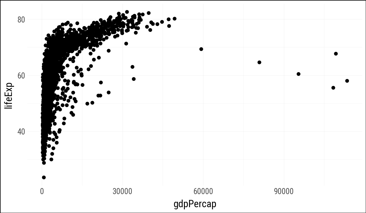
        ('gdpPercap', Float64)])

2.4 Make Your First Figure

(
    gapminder
    .ggplot(aes(x="gdpPercap", y="lifeExp"))
    .geom_point()
)

Figure 2.1: Life expectancy plotted against GDP per capita for a large number of country-years.

Joel Grus has an entertaining discussion of the problems with notebooks, some of which are addressed by Quarto documents.↩︎