Chapter 4 examines the fascinating topic of cohorts, where a cohort is a group of observations (often people) who acquire a shared characteristic at (approximately) the same time. For example, children entering kindergarten in New Zealand in 2017 or the Harvard MBA Class of 2002.
While cohort analysis has some attractive features, I guess that data do not often come in a format that facilitates such analysis. Instead, as is the case with the legislators data set studied in Chapter 4, the data analyst needs to rearrange the data to support cohort analysis.
I found Chapter 4 a little confusing on a first pass through it.1 The chapter launches into some SQL code intended to create cohorts, but it’s a little unclear why we’re doing what we’re doing, and we quickly see that our cohort analysis does not make sense (e.g., we have more of our original cohort in period 5 than we had in period 4) and we must have done something wrong. I think I see the idea Cathy is going for here: one needs to think carefully about how to arrange the data to avoid subtle mistakes. The challenge I see is that it’s not obvious that everyone would make the same mistake and one is too deep in the weeds of the code to really see the forest for the trees.
So before I launch into the code, I will spend a little time thinking about things conceptually. I will start with a different example from that used in Chapter 4, but one that I think brings out some of the issues.
For some reason I associate cohort analysis with life expectancy. The people who are born today form a cohort and one might ask: How long do we expect members of this cohort to live? One often hears life expectancy statistics quoted as something like: “In Australia, a boy born in 2018–2020 can expect to live to the age of 81.2 years and a girl would be expected to live to 85.3 years compared to 51.1 for boys and 54.8 years for girls born in in 1891–1900.”2
The people who construct the life expectancies for the children must be veritable polymaths. They need to anticipate future developments in medical care and technology. Skin cancer is a significant cause of death in Australia, due to a mismatch between the median complexion and the intensity of the sun. But the analysts calculating life expectancy need to think about how medical technology is likely to affect rates of death from carcinoma in the future. I can imagine whole-body scanners a bit like the scanners in US airports that detect skin cancers before they become problematic. These analysts also need to understand how road safety will evolve. Will children today all be in driverless vehicles in fifty years time and will accidents then be a rarity? And what about war? The data analyst needs to be able to forecast the possibility of World War III breaking out and shortening life spans. Who are these people?
Of course it seems unlikely these über-analysts exist. Rather they surely do something more prosaic. Here is my guess as to how life expectancies are constructed.3 I guess that the data analyst gathers data on cohorts notionally formed at some point in the past and then looks at survival rates for that cohort over some period, then aggregates those data into a life expectancy.
For example, the data analyst might gather data on people who turned 21 in 2018 and then data on whether those people surived to their 22nd birthday. The proportion of such people who make their 22nd birthday could be interpreted as a survival probability \(p_{21}\). Repeat that for each age-based cohort to get probabilities \(\left\{p_i: i = 0, 1, \dots, 119, 120 \right\}\). Now to find the median life expectancy, we could calculate something like this:4
\[ \left\{j: \arg \min_{i} \left(\prod_{0}^{i} p_i\right) \leq \frac{1}{2} \right\} \] So we have a (fairly) well-defined procedure here. There are obviously some details to be worked out. For example, do we focus on one year (2018 in this case)? Or collect data over multiple years? Does it make sense to form cohorts by years? Or would grouping into larger cohorts (e.g., 20–25) make more sense? Do we identify people by birthdays? Or just use some kind of census date? (People who are 21 on 1 July might have just turned 21, or might be about to turn 22.)
But what exactly have we calculated? In a sense it’s a nonsensical number. Why would survival rates for 88-year-olds in 2018 be relevant for the life expectancy of newborns today, who will face a very different world when they turn 88 in 2111. First, perhaps the analysts really don’t calculate it in this way (though I’m doubtful they are polymaths). Second, even though it’s a “meaningless” number, it probably still has attractive properties, such as the ability to represent in a one or two numbers a lot about the quality of life in Australia.
A final note is that it is not clear to me where the “51.1 for boys and 54.8 years for girls born in in 1891–1900” values come from. Are these the equivalent life expectancies calculated using data available around 1900? Or are these the observed lifespans of people born in 1891–1900? If the latter, how accurate were the former as estimates of these values?
db <-dbConnect(duckdb::duckdb())legislators <-tbl(db, "read_csv_auto('data/legislators.csv')") |>compute(name ="legislators")legislators_terms <-tbl(db, "read_csv_auto('data/legislators_terms.csv')") |>compute(name ="legislators_terms")
4.2.2 Exploring the data
There are two tables in the legislators data set. The legislators data looks to have id_bioguide as a primary key.
WITHid_rows AS (SELECT id_bioguide, count(*) AS rows_per_idFROM legislatorsGROUPBY1)SELECT rows_per_id, count(*) AS num_idsFROM id_rowsGROUPBY1;
1 records
rows_per_id
num_ids
1
12518
SELECTCOUNT(*) AS num_missing_idsFROM legislatorsWHERE id_bioguide ISNULL
1 records
num_missing_ids
0
WITH id_rows AS (SELECT id_bioguide, term_start,count(*) AS rows_per_idFROM legislators_termsGROUPBY1, 2)SELECT rows_per_id, count(*) AS num_idsFROM id_rowsGROUPBY1;
1 records
rows_per_id
num_ids
1
44063
SELECTCOUNT(*) AS num_missing_idsFROM legislators_termsWHERE id_bioguide ISNULLOR term_start ISNULL
1 records
num_missing_ids
0
WITH id_rows AS (SELECT id_bioguide, term_number,count(*) AS rows_per_idFROM legislators_termsGROUPBY1, 2)SELECT rows_per_id, count(*) AS num_idsFROM id_rowsGROUPBY1;
1 records
rows_per_id
num_ids
1
44063
SELECTCOUNT(*) AS num_missing_idsFROM legislators_termsWHERE term_end ISNULL
1 records
num_missing_ids
0
SELECTmax(term_start) AS max_term_start,max(term_end) AS max_term_endFROM legislators_terms
Clearly we have term_end dates that are anticipated based on
4.3 Retention
4.3.1 SQL for a Basic Retention Curve
SELECT id_bioguide, min(term_start) AS first_termFROM legislators_terms GROUPBY1LIMIT3;
3 records
id_bioguide
first_term
F000062
1992-11-10
T000464
2007-01-04
A000360
2003-01-07
WITH first_terms AS (SELECT id_bioguide, min(term_start) AS first_termFROM legislators_terms GROUPBY1) SELECT date_part('year', age(b.term_start, a.first_term)) AS period,COUNT(DISTINCT a.id_bioguide) AS cohort_retainedFROM first_terms aINNERJOIN legislators_terms bUSING (id_bioguide)GROUPBY1ORDERBY1LIMIT4;
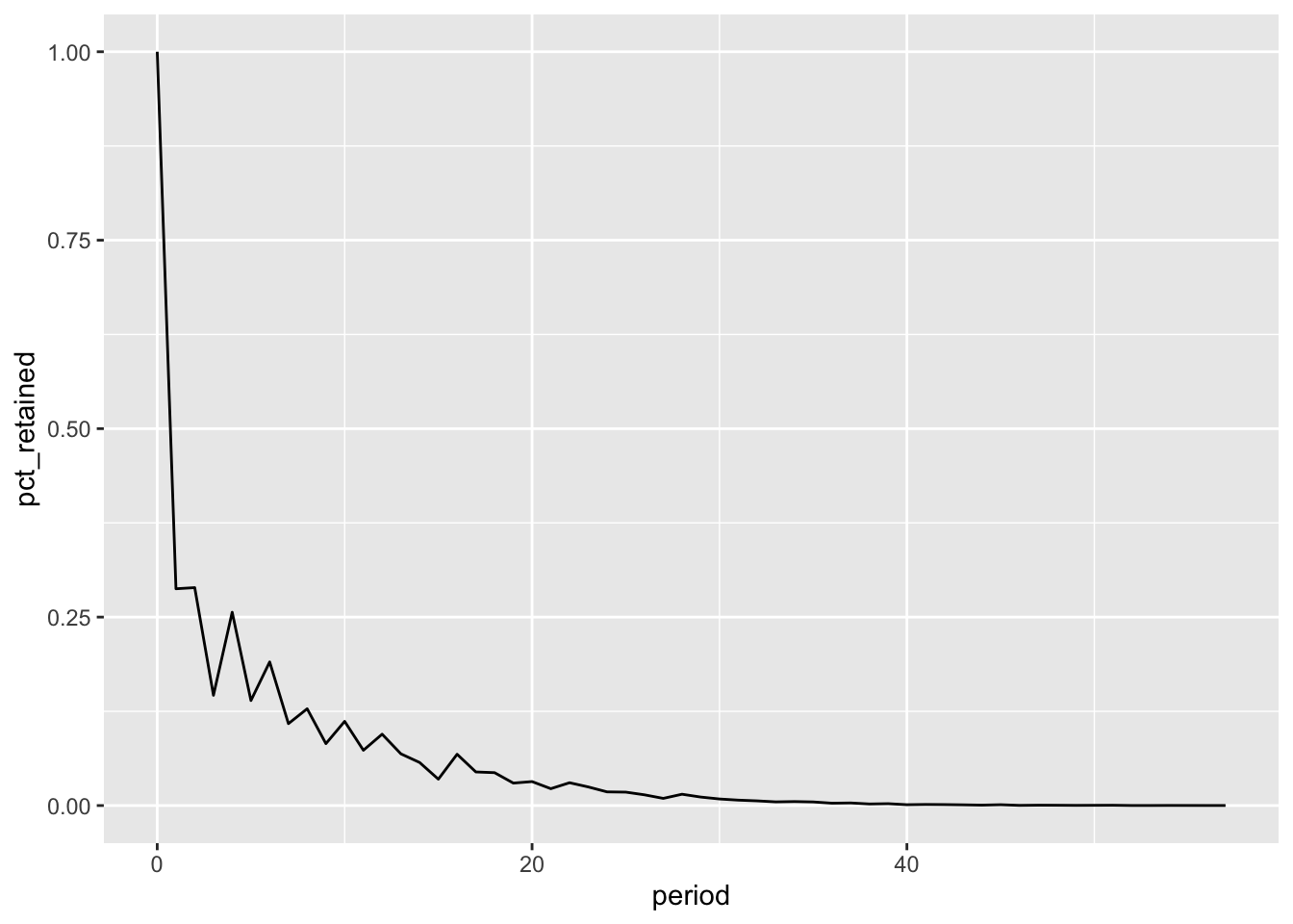
WITHfirst_terms AS (SELECT id_bioguide, min(term_start) AS first_termFROM legislators_terms GROUPBY1),cohorts AS (SELECT date_part('year', age(b.term_start, a.first_term)) AS period,COUNT(DISTINCT a.id_bioguide) AS cohort_retainedFROM first_terms aJOIN legislators_terms b USING (id_bioguide)GROUPBY1)SELECT period,first_value(cohort_retained) OVER w AS cohort_size, cohort_retained, cohort_retained *1.0/first_value(cohort_retained) OVER w AS prop_retainedFROM cohortsWINDOW w AS (ORDERBY period)LIMIT3;
retained_data |>ggplot(aes(x = period, y = pct_retained)) +geom_line()
WITHfirst_terms AS (SELECT id_bioguide, min(term_start) AS first_termFROM legislators_terms GROUPBY1),cohorts AS (SELECT date_part('year', age(b.term_start, a.first_term)) AS period,COUNT(DISTINCT a.id_bioguide) AS cohort_retainedFROM first_terms aJOIN legislators_terms b on a.id_bioguide = b.id_bioguide GROUPBY1),retained_data AS (SELECT period,first_value(cohort_retained) OVER w AS cohort_size, cohort_retained, cohort_retained *1.0/first_value(cohort_retained) OVER w AS pct_retainedFROM cohorts WINDOW w AS (ORDERBY period))SELECT cohort_size,max(CASEWHEN period =0THEN pct_retained END) AS yr0,max(CASEWHEN period =1THEN pct_retained END) AS yr1,max(CASEWHEN period =2THEN pct_retained END) AS yr2,max(CASEWHEN period =3THEN pct_retained END) AS yr3,max(CASEWHEN period =4THEN pct_retained END) AS yr4FROM retained_dataGROUPBY1;
4.3.2 Adjusting Time Series to Increase Retention Accuracy
Use copy_inline() here if using a read-only database.
year_ends <-tibble(date =seq(as.Date('1770-12-31'), as.Date('2030-12-31'), by ="1 year")) |>copy_to(db, df = _, overwrite =TRUE, name ="year_ends")
WITHfirst_terms AS (SELECT id_bioguide, min(term_start) AS first_termFROM legislators_terms GROUPBY1)SELECT a.id_bioguide, a.first_term, b.term_start, b.term_end, c.date, date_part('year', age(c.date, a.first_term)) AS periodFROM first_terms aJOIN legislators_terms b USING (id_bioguide)LEFTJOIN year_ends cON c.dateBETWEEN b.term_start and b.term_endORDERBY id_bioguideLIMIT3;
WITHfirst_terms AS (SELECT id_bioguide, min(term_start) AS first_termFROM legislators_terms GROUPBY1),cohorts_retained AS ( SELECTcoalesce(date_part('year', age(c.date, a.first_term)), 0) AS period,COUNT(DISTINCT a.id_bioguide) AS cohort_retainedFROM first_terms aJOIN legislators_terms bUSING (id_bioguide)LEFTJOIN year_ends c ON c.dateBETWEEN b.term_start AND b.term_endGROUPBY1)SELECT period,first_value(cohort_retained) OVER w AS cohort_size, cohort_retained, cohort_retained *1.0/first_value(cohort_retained) OVER w AS pct_retainedFROM cohorts_retainedWINDOW w AS (ORDERBY period);
For now, I have omitted the query after the paragraph starting “A second option …”.
4.3.3 Cohorts Derived from the Time Series Itself
WITH first_terms AS (SELECT id_bioguide, min(term_start) AS first_termFROM legislators_terms GROUPBY1)SELECT date_part('year', a.first_term) AS first_year,COALESCE(date_part('year', age(c.date, a.first_term)), 0) AS period,COUNT(DISTINCT a.id_bioguide) AS cohort_retainedFROM first_terms aINNERJOIN legislators_terms b USING (id_bioguide)LEFTJOIN year_ends c ON c.dateBETWEEN b.term_start AND b.term_end GROUPBY1, 2ORDERBY1, 2LIMIT3;
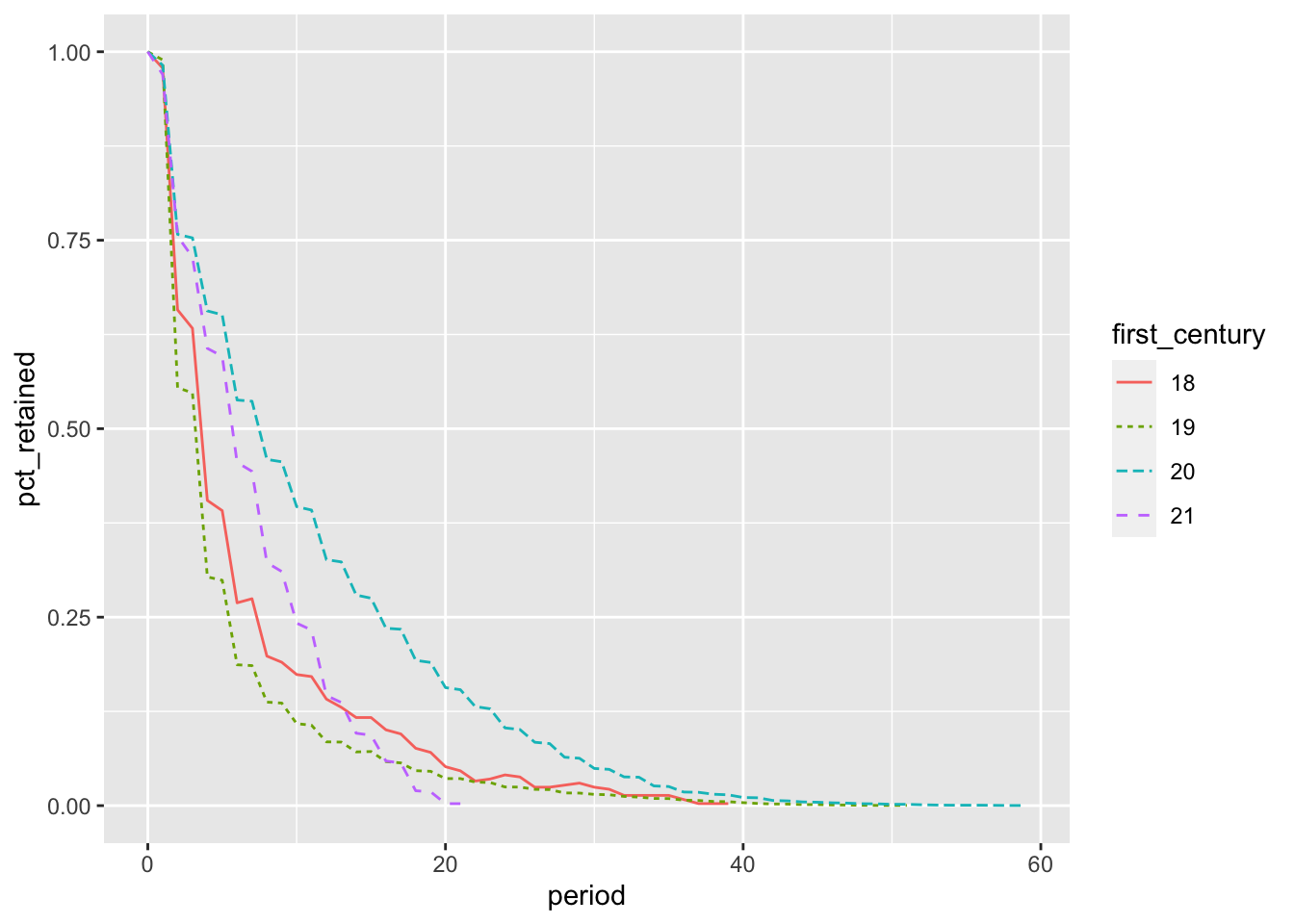
WITH first_terms AS (SELECT id_bioguide, min(term_start) AS first_termFROM legislators_terms GROUPBY1),first_centuries AS (SELECT date_part('century', a.first_term) AS first_century,coalesce(date_part('year', age(c.date, a.first_term)), 0) AS period,COUNT(DISTINCT a.id_bioguide) AS cohort_retainedFROM first_terms AS aINNERJOIN legislators_terms b USING (id_bioguide)LEFTJOIN year_ends c ON c.dateBETWEEN b.term_start AND b.term_end GROUPBY1, 2)SELECT first_century, period,first_value(cohort_retained) OVER w AS cohort_size, cohort_retained, cohort_retained *1.0/first_value(cohort_retained) OVER w AS prop_retainedFROM first_centuriesWINDOW w AS (PARTITIONBY first_century ORDERBY period)ORDERBY1, 2LIMIT3;
SELECTDISTINCT id_bioguide,min(term_start) OVER w AS first_term,first_value(state) OVER w AS first_stateFROM legislators_terms WINDOW w AS (PARTITIONBY id_bioguide ORDERBY term_start)ORDERBY id_bioguide
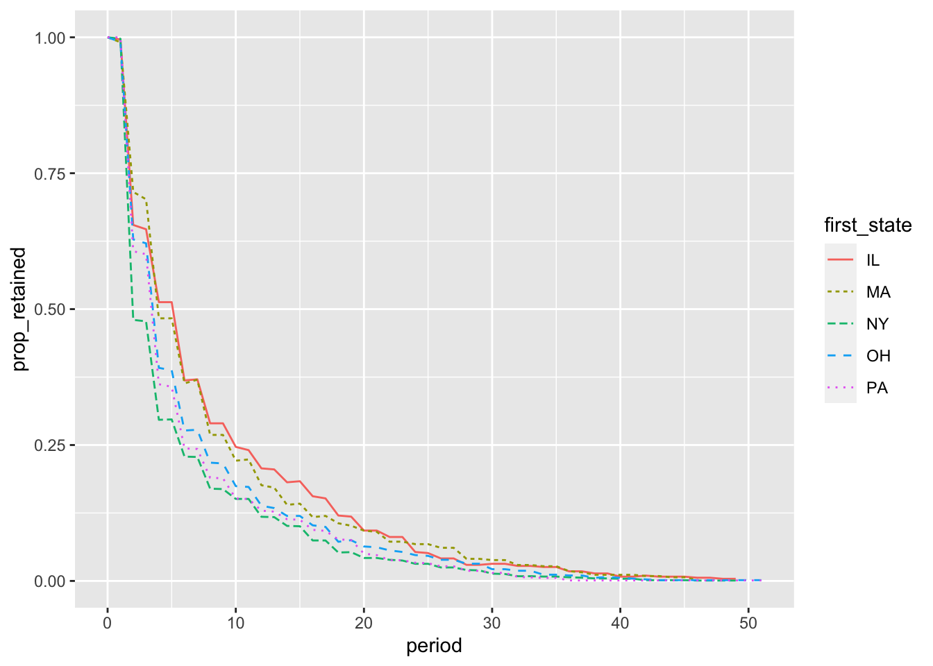
WITH first_states AS (SELECTDISTINCT id_bioguide,min(term_start) OVER w AS first_term,first_value(state) OVER w AS first_stateFROM legislators_terms WINDOW w AS (PARTITIONBY id_bioguide ORDERBY term_start)),state_first_periods AS (SELECT first_state,coalesce(date_part('year', age(c.date, a.first_term)), 0) AS period,COUNT(DISTINCT a.id_bioguide) AS cohort_retainedFROM first_states AS aINNERJOIN legislators_terms b USING (id_bioguide)LEFTJOIN year_ends c ON c.dateBETWEEN b.term_start AND b.term_end GROUPBY1, 2)SELECT first_state, period,first_value(cohort_retained) OVER w AS cohort_size, cohort_retained, cohort_retained *1.0/first_value(cohort_retained) OVER w AS prop_retainedFROM state_first_periodsWINDOW w AS (PARTITIONBY first_state ORDERBY period)ORDERBY1, 2LIMIT3;
WITH first_terms AS (SELECT id_bioguide, min(term_start) AS first_termFROM legislators_terms GROUPBY1)SELECT d.gender,coalesce(date_part('year',age(c.date,a.first_term)),0) AS period,count(distinct a.id_bioguide) AS cohort_retainedFROM first_terms aJOIN legislators_terms b ON a.id_bioguide = b.id_bioguide LEFTJOIN year_ends c ON c.dateBETWEEN b.term_start AND b.term_end INNERJOIN legislators d ON a.id_bioguide = d.id_bioguideGROUPBY1,2ORDERBY2,1LIMIT4;
WITH first_terms AS (SELECT id_bioguide, min(term_start) AS first_termFROM legislators_terms GROUPBY1),cohorts AS (SELECT d.gender,coalesce(date_part('year',age(c.date,a.first_term)),0) as period,count(distinct a.id_bioguide) as cohort_retainedFROM first_terms aJOIN legislators_terms b on a.id_bioguide = b.id_bioguide LEFTJOIN year_ends c on c.datebetween b.term_start and b.term_end JOIN legislators d on a.id_bioguide = d.id_bioguideGROUPBY1, 2)SELECT gender, period, cohort_retained,first_value(cohort_retained) OVER w AS cohort_size, cohort_retained *1.0/first_value(cohort_retained) OVER w AS pct_retainedFROM cohorts aaWINDOW w AS (partitionby gender orderby period)ORDERBY2, 1LIMIT4;
WITH first_terms AS (SELECT id_bioguide, min(term_start) AS first_termFROM legislators_terms GROUPBY1),cohorts AS (SELECT d.gender,coalesce(date_part('year',age(c.date, a.first_term)),0) as period,count(distinct a.id_bioguide) as cohort_retainedFROM first_terms aJOIN legislators_terms b on a.id_bioguide = b.id_bioguide LEFTJOIN year_ends c on c.datebetween b.term_start and b.term_end JOIN legislators d on a.id_bioguide = d.id_bioguideWHERE first_term BETWEEN'1917-01-01'AND'1999-12-31'GROUPBY1, 2)SELECT gender, period, cohort_retained,first_value(cohort_retained) OVER w AS cohort_size, cohort_retained *1.0/first_value(cohort_retained) OVER w AS pct_retainedFROM cohorts aaWINDOW w AS (PARTITIONBY gender ORDERBY period)ORDERBY2, 1LIMIT4;
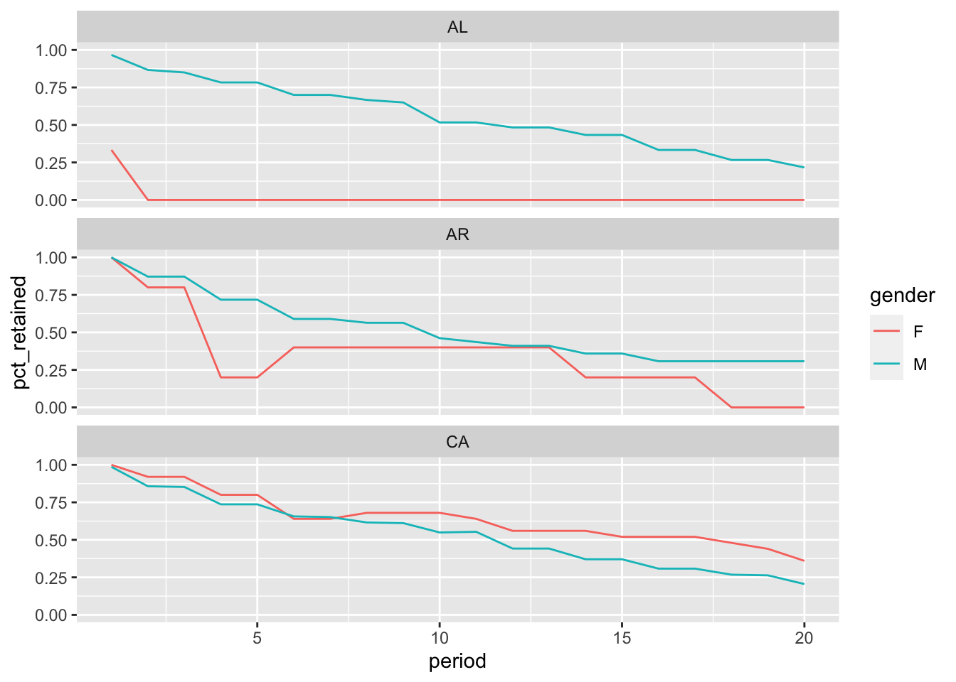
WITHfirst_terms AS (SELECT id_bioguide, min(term_start) AS term_start,FROM legislators_termsGROUPBY1),first_states AS (SELECT id_bioguide, gender, term_start AS first_term, state AS first_stateFROM first_termsINNERJOIN legislators_termsUSING (id_bioguide, term_start)INNERJOIN legislatorsUSING (id_bioguide)WHERE term_start between'1917-01-01'and'1999-12-31'),cohorts AS (SELECT first_state, gender,coalesce(date_part('year', age(date, first_term)), 0) AS period,COUNT(DISTINCT id_bioguide) AS cohort_retainedFROM first_statesINNERJOIN legislators_termsUSING (id_bioguide)LEFTJOIN year_endsONdateBETWEEN term_start AND term_endGROUPBY1, 2, 3),periods AS (SELECT generate_series as period FROM generate_series(0, 20, 1)),cohort_sizes AS (SELECT gender, first_state,COUNT(DISTINCT id_bioguide) AS cohort_sizeFROM first_statesGROUPBY1, 2),pct_retaineds AS (SELECT gender, first_state, period, cohort_size,coalesce(cohort_retained, 0) AS cohort_retained,coalesce(cohort_retained, 0) *1.0/ cohort_size AS pct_retainedFROM cohort_sizesCROSSJOIN periodsLEFTJOIN cohortsUSING (gender, first_state, period))SELECT gender, first_state, cohort_size,max(casewhen period =0then pct_retained end) as yr0,max(casewhen period =2then pct_retained end) as yr2,max(casewhen period =4then pct_retained end) as yr4,max(casewhen period =6then pct_retained end) as yr6,max(casewhen period =8then pct_retained end) as yr8,max(casewhen period =10then pct_retained end) as yr10FROM pct_retainedsWHERE first_state IN ('AL', 'AR', 'CA')GROUPBY1, 2, 3ORDERBY1, 2LIMIT3;
Does this mean something is wrong with our query? Let’s check.
Of course, unlike cohorts of living people, dropping out of the cohort of legislators does not prevent you from returning later on. We can pull out a portion of the query creating cohorts and take a closer look. We first get the id_bioguide values for the female representatives from Arkansas (AR) who are around in period == 4. We then look at some data from legislators and legislators_terms for these two representatives.
From the above, it seems that Blanche Lambert Lincoln would have dropped out of the cohort in periods 4 and 5, then returned in 6 and 7.
To aid this kind of “debugging” of our queries, we could easily have retained some underlying data in cohorts. For example, by added cohort_ids = array_agg(id_bioguide) to the query, we can easily interrogate cohorts for the underlying legislator IDs.
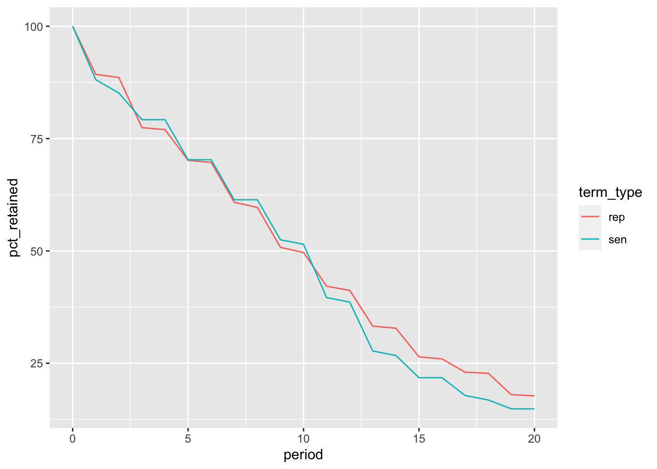
4.3.6 Defining Cohorts from Dates other than the First Date
WITH first_terms AS (SELECTDISTINCT id_bioguide, term_type,'2000-01-01'::dateAS first_term,min(term_start) AS min_startFROM legislators_terms WHERE term_start <='2000-12-31'and term_end >='2000-01-01'GROUPBY1, 2, 3),cohort_dates AS (SELECT id_bioguide, dateFROM legislators_termsLEFTJOIN year_ends ONdateBETWEEN term_start AND term_end),cohorts AS (SELECT term_type,coalesce(date_part('year', age(date, first_term)), 0) AS period,COUNT(DISTINCT id_bioguide) AS cohort_retainedFROM first_termsJOIN cohort_datesUSING (id_bioguide)GROUPBY1, 2)SELECT term_type, period,first_value(cohort_retained) OVER w AS cohort_size, cohort_retained, cohort_retained *1.0/first_value(cohort_retained) OVER w AS pct_retainedFROM cohortsWHERE period >=0WINDOW w AS (PARTITIONBY term_type ORDERBY period)ORDERBY2, 1LIMIT4;
pct_retained_2000 |>filter(period <=20) |>mutate(pct_retained = pct_retained *100) |>ggplot(aes(x = period, y = pct_retained,colour = term_type, group = term_type)) +geom_line()
4.4 Related Cohort Analyses
4.4.1 Survivorship
WITH first_centuries AS (SELECT id_bioguide, date_part('century', min(term_start)) AS first_century,min(term_start) AS first_term,max(term_start) AS last_term, date_part('year', age(max(term_start), min(term_start))) AS tenureFROM legislators_termsGROUPBY1)SELECT first_century,count(distinct id_bioguide) as cohort_size,count(distinctcasewhen tenure >=10then id_bioguide end) as survived_10,count(distinctcasewhen tenure >=10then id_bioguide end) *1.0/count(distinct id_bioguide) as pct_survived_10FROM first_centuriesGROUPBY1ORDERBY1;
4 records
first_century
cohort_size
survived_10
pct_survived_10
18
368
83
0.2255435
19
6299
892
0.1416098
20
5091
1853
0.3639756
21
760
119
0.1565789
WITH first_centuries AS (SELECT id_bioguide, date_part('century', min(term_start)) AS first_century,count(term_start) AS total_termsFROM legislators_termsGROUPBY1)SELECT first_century,COUNT(DISTINCT id_bioguide) AS cohort_size,COUNT(DISTINCTCASEWHEN total_terms >=5THEN id_bioguide END) AS survived_5,COUNT(DISTINCTCASEWHEN total_terms >=5THEN id_bioguide END) *1.0/count(distinct id_bioguide) AS pct_survived_5_termsFROM first_centuriesGROUPBY1ORDERBY1;
4 records
first_century
cohort_size
survived_5
pct_survived_5_terms
18
368
63
0.1711957
19
6299
711
0.1128751
20
5091
2153
0.4229032
21
760
205
0.2697368
WITH first_centuries AS (SELECT id_bioguide, date_part('century',min(term_start)) AS first_century,count(term_start) AS total_termsFROM legislators_termsGROUPBY1),terms AS (SELECT generate_series as terms FROM generate_series(1, 20, 1))SELECT first_century, terms,count(distinct id_bioguide) as cohort,count(distinctcasewhen total_terms >= terms then id_bioguide end) as cohort_survived,count(distinctcasewhen total_terms >= terms then id_bioguide end) *1.0/count(distinct id_bioguide) as pct_survivedFROM first_centuriesCROSSJOIN termsGROUPBY1, 2ORDERBY first_century, termsLIMIT3;
WITH rep_first_terms AS (SELECT id_bioguide, min(term_start) AS first_termFROM legislators_termsWHERE term_type ='rep'GROUPBY1)SELECT date_part('century', first_term)::intAS cohort_century,count(id_bioguide) AS repsFROM rep_first_termsGROUPBY1ORDERBY1
4 records
cohort_century
reps
18
299
19
5773
20
4481
21
683
WITH rep_first_terms AS (SELECT id_bioguide, min(term_start) AS first_termFROM legislators_termsWHERE term_type ='rep'GROUPBY1)SELECT date_part('century', first_term) AS cohort_century,count(id_bioguide) as repsFROM rep_first_termsGROUPBY1ORDERBY1;
4 records
cohort_century
reps
18
299
19
5773
20
4481
21
683
WITH rep_first_terms AS (SELECT id_bioguide, min(term_start) AS first_termFROM legislators_termsWHERE term_type ='rep'GROUPBY1),num_reps AS (SELECT date_part('century', first_term) as cohort_century,count(id_bioguide) as repsFROM rep_first_termsGROUPBY1),sens AS (SELECT date_part('century',b.first_term) as cohort_century,count(distinct b.id_bioguide) as rep_and_senFROM rep_first_terms bJOIN legislators_terms c on b.id_bioguide = c.id_bioguideand c.term_type ='sen'and c.term_start > b.first_termGROUPBY1)SELECT aa.cohort_century, bb.rep_and_sen *1.0/ aa.reps as pct_rep_and_senFROM num_reps aaLEFTJOIN sens bb on aa.cohort_century = bb.cohort_century;
4 records
cohort_century
pct_rep_and_sen
20
0.0566838
21
0.0366032
18
0.1906355
19
0.0569894
WITHrep_first_terms AS (SELECT id_bioguide, min(term_start) AS first_termFROM legislators_termsWHERE term_type ='rep'GROUPBY1),reps AS (SELECT date_part('century',a.first_term) as cohort_century,count(id_bioguide) as repsFROM rep_first_terms aWHERE first_term <='2009-12-31'GROUPBY1),sens AS (SELECT date_part('century',b.first_term) as cohort_century,count(distinct b.id_bioguide) as rep_and_senFROM rep_first_terms bJOIN legislators_terms c on b.id_bioguide = c.id_bioguideand c.term_type ='sen'and c.term_start > b.first_termWHERE age(c.term_start, b.first_term) <=interval'10 years'GROUPBY1)SELECT aa.cohort_century,bb.rep_and_sen *1.0/ aa.reps as pct_rep_and_senFROM reps aaLEFTJOIN sens bb USING (cohort_century);
4 records
cohort_century
pct_rep_and_sen
20
0.0348137
21
0.0763636
18
0.0969900
19
0.0244240
WITHrep_first_terms AS (SELECT id_bioguide, min(term_start) AS first_termFROM legislators_termsWHERE term_type ='rep'GROUPBY1),reps AS (SELECT date_part('century', first_term) as cohort_century,count(id_bioguide) as repsFROM rep_first_termsWHERE first_term <='2009-12-31'GROUPBY1),sen_terms AS (SELECT id_bioguide, term_type, term_startFROM legislators_termsWHERE term_type ='sen'),gaps AS (SELECT id_bioguide, first_term, age(term_start, first_term) AS gapFROM rep_first_terms JOIN sen_terms USING (id_bioguide)WHERE term_start > first_term),gap_indicators AS (SELECT date_part('century', first_term) as cohort_century,count(distinctcasewhen gap <=interval'5 years'then id_bioguide end) as rep_and_sen_5_yrs,count(distinctcasewhen gap <=interval'10 years'then id_bioguide end) as rep_and_sen_10_yrs,count(distinctcasewhen gap <=interval'15 years'then id_bioguide end) as rep_and_sen_15_yrsFROM gapsGROUPBY1)SELECT cohort_century::intas cohort_century,round(rep_and_sen_5_yrs *1.0/ reps, 4) as pct_5_yrs,round(rep_and_sen_10_yrs *1.0/ reps, 4) as pct_10_yrs,round(rep_and_sen_15_yrs *1.0/ reps, 4) as pct_15_yrsFROM repsLEFTJOIN gap_indicatorsUSING (cohort_century)ORDERBY cohort_century
4 records
cohort_century
pct_5_yrs
pct_10_yrs
pct_15_yrs
18
0.0502
0.0970
0.1438
19
0.0088
0.0244
0.0409
20
0.0100
0.0348
0.0478
21
0.0400
0.0764
0.0873
4.4.3 Cumulative Calculations
WITHtypesAS (SELECTdistinct id_bioguide,first_value(term_type) over w as first_type,min(term_start) over w as first_term, (min(term_start) over w) +interval'10 years'as first_plus_10FROM legislators_terms WINDOW w AS (partitionby id_bioguide orderby term_start))SELECT date_part('century',a.first_term)::intas century, first_type,count(distinct a.id_bioguide) as cohort,count(b.term_start) as termsFROMtypes aLEFTJOIN legislators_terms b on a.id_bioguide = b.id_bioguide and b.term_start between a.first_term and a.first_plus_10GROUPBY1, 2;
8 records
century
first_type
cohort
terms
20
rep
4473
16203
19
rep
5744
12165
20
sen
618
1008
19
sen
555
795
18
sen
71
101
21
sen
77
118
21
rep
683
2203
18
rep
297
760
WITH a AS (SELECTDISTINCT id_bioguide,first_value(term_type) OVER w AS first_type,min(term_start) OVER w AS first_termFROM legislators_terms WINDOW w AS (PARTITIONBY id_bioguide ORDERBY term_start)),cohort_terms AS (SELECT date_part('century',a.first_term)::intAS century, first_type,COUNT(distinct a.id_bioguide) AS cohort,COUNT(b.term_start) as terms,COUNT(b.term_start) *1.0/COUNT(DISTINCT a.id_bioguide) AS cohort_termFROM aLEFTJOIN legislators_terms b on a.id_bioguide = b.id_bioguide AND b.term_start BETWEEN a.first_term AND a.first_term +interval'10 years'GROUPBY1, 2)SELECT century,max(casewhen first_type ='rep'then cohort end) as rep_cohort,max(casewhen first_type ='rep'then cohort_term end) as avg_rep_terms,max(casewhen first_type ='sen'then cohort end) as sen_cohort,max(casewhen first_type ='sen'then cohort_term end) as avg_sen_termsFROM cohort_termsGROUPBY1;
4 records
century
rep_cohort
avg_rep_terms
sen_cohort
avg_sen_terms
20
4473
3.622401
618
1.631068
19
5744
2.117862
555
1.432432
21
683
3.225476
77
1.532468
18
297
2.558923
71
1.422535
4.5 Cross-Section Analysis, Through a Cohort Lens
SELECT b.date, count(distinct a.id_bioguide) as legislatorsFROM legislators_terms aJOIN year_ends b on b.datebetween a.term_start and a.term_endand b.date<='2020-12-31'GROUPBY1;
Displaying records 1 - 10
date
legislators
1855-12-31
306
1856-12-31
306
1853-12-31
315
1854-12-31
316
1851-12-31
303
1852-12-31
310
1849-12-31
310
1850-12-31
313
1848-12-31
306
1847-12-31
301
SELECT b.date,date_part('century',first_term)::intas century,count(distinct a.id_bioguide) as legislatorsFROM legislators_terms aJOIN year_ends b on b.datebetween a.term_start and a.term_endand b.date<='2020-12-31'JOIN(SELECT id_bioguide, min(term_start) as first_termFROM legislators_termsGROUPBY1) c on a.id_bioguide = c.id_bioguide GROUPBY1,2;
Displaying records 1 - 10
date
century
legislators
1919-12-31
20
516
1965-12-31
20
546
1995-12-31
20
539
2005-12-31
20
388
1975-12-31
20
547
1811-12-31
19
153
1893-12-31
19
470
1909-12-31
20
344
1937-12-31
20
547
2010-12-31
21
262
SELECTdate,century,legislators,sum(legislators) over (partitionbydate) as cohort,legislators *100.0/sum(legislators) over (partitionbydate) as pct_centuryFROM(SELECT b.date ,date_part('century',first_term)::intas century ,count(distinct a.id_bioguide) as legislatorsFROM legislators_terms aJOIN year_ends b on b.datebetween a.term_start and a.term_endand b.date<='2020-01-01'JOIN (SELECT id_bioguide, min(term_start) as first_termFROM legislators_termsGROUPBY1 ) c on a.id_bioguide = c.id_bioguide GROUPBY1,2) aORDERBY1,2;
Displaying records 1 - 10
date
century
legislators
cohort
pct_century
1789-12-31
18
89
89
100
1790-12-31
18
95
95
100
1791-12-31
18
99
99
100
1792-12-31
18
101
101
100
1793-12-31
18
141
141
100
1794-12-31
18
140
140
100
1795-12-31
18
145
145
100
1796-12-31
18
150
150
100
1797-12-31
18
152
152
100
1798-12-31
18
155
155
100
WITHfirst_terms AS (SELECT id_bioguide, min(term_start) as first_termFROM legislators_termsGROUPBY1),aa AS (SELECT b.date, date_part('century',first_term)::intas century,count(distinct a.id_bioguide) as legislatorsFROM legislators_terms aJOIN year_ends b ON b.datebetween a.term_start and a.term_endand b.date<='2020-01-01'JOIN first_terms c USING (id_bioguide)GROUPBY1,2) SELECTdate,coalesce(sum(casewhen century =18then legislators end) *100.0/sum(legislators),0) as pct_18,coalesce(sum(casewhen century =19then legislators end) *100.0/sum(legislators),0) as pct_19,coalesce(sum(casewhen century =20then legislators end) *100.0/sum(legislators),0) as pct_20,coalesce(sum(casewhen century =21then legislators end) *100.0/sum(legislators),0) as pct_21FROM aaGROUPBY1ORDERBY1;
Displaying records 1 - 10
date
pct_18
pct_19
pct_20
pct_21
1789-12-31
100
0
0
0
1790-12-31
100
0
0
0
1791-12-31
100
0
0
0
1792-12-31
100
0
0
0
1793-12-31
100
0
0
0
1794-12-31
100
0
0
0
1795-12-31
100
0
0
0
1796-12-31
100
0
0
0
1797-12-31
100
0
0
0
1798-12-31
100
0
0
0
SELECT id_bioguide, date,count(date) over (partitionby id_bioguide orderbydaterowsbetweenunboundedprecedingandcurrentrow) as cume_yearsFROM (SELECTdistinct id_bioguide, dateFROM legislators_termsJOIN year_ends ONdatebetween term_start and term_endanddate<='2020-01-01');
Displaying records 1 - 10
id_bioguide
date
cume_years
A000009
1973-12-31
1
A000009
1974-12-31
2
A000009
1975-12-31
3
A000009
1976-12-31
4
A000009
1977-12-31
5
A000009
1978-12-31
6
A000009
1979-12-31
7
A000009
1980-12-31
8
A000009
1981-12-31
9
A000009
1982-12-31
10
SELECTdate, cume_years,count(distinct id_bioguide) as legislatorsFROM(SELECT id_bioguide, date ,count(date) over (partitionby id_bioguide orderbydaterowsbetweenunboundedprecedingandcurrentrow) as cume_yearsFROM (SELECTdistinct a.id_bioguide, b.dateFROM legislators_terms aJOIN year_ends b on b.datebetween a.term_start and a.term_end and b.date<='2020-01-01'GROUPBY1,2 ) aa) aaaGROUPBY1,2;
Displaying records 1 - 10
date
cume_years
legislators
1995-12-31
17
30
1999-12-31
5
68
2018-12-31
6
71
1988-12-31
2
54
1978-12-31
2
79
1903-12-31
7
75
2018-12-31
2
61
1948-12-31
3
10
1868-12-31
2
119
1999-12-31
9
30
WITH aa AS (SELECTDISTINCT a.id_bioguide, b.dateFROM legislators_terms aJOIN year_ends b on b.dateBETWEEN a.term_start AND a.term_end AND b.date<='2020-01-01'GROUPBY1,2),aaa AS (SELECT id_bioguide, date,count(date) OVER (PARTITIONBY id_bioguide ORDERBYdate) AS cume_yearsFROM aa),aaaa AS (SELECTdate, cume_years,COUNT(DISTINCT id_bioguide) as legislatorsFROM aaaGROUPBY1,2)SELECTdate, count(*) as tenuresFROM aaaaGROUPBY1;
Displaying records 1 - 10
date
tenures
1973-12-31
35
1974-12-31
36
1975-12-31
36
1976-12-31
36
1977-12-31
34
1978-12-31
34
1979-12-31
31
1980-12-31
32
1981-12-31
31
1982-12-31
32
WITH term_dates AS (SELECTdistinct a.id_bioguide, b.dateFROM legislators_terms aJOIN year_ends b on b.datebetween a.term_start and a.term_end and b.date<='2020-01-01'),cum_term_dates AS (SELECT id_bioguide, date,count(date) over (partitionby id_bioguide orderbydaterowsbetweenunboundedprecedingandcurrentrow) as cume_yearsFROM term_dates),cum_term_bands AS (SELECTdate,casewhen cume_years <=4then'1 to 4'when cume_years <=10then'5 to 10'when cume_years <=20then'11 to 20'else'21+'endas tenure,count(distinct id_bioguide) as legislatorsFROM cum_term_datesGROUPBY1,2)SELECTdate, tenure, legislators *100.0/sum(legislators) over w as pct_legislators FROM cum_term_bandsWINDOW w AS (partitionbydate)ORDERBYdateDESC;
I made no effort to research how they are constructed because (1) I am lazy and (2) my imagined version is probably better for my current purposes.↩︎
There are some details I’m glossing over here, such as the fact that there will be some \(j\) where the cumulative survival probability is just above one-half, but where that for \(j + 1\) is just below one-half, so some interpolation will be required.↩︎