Geometric Objects

This notebook adapts the plotnine guide on geometric objects to the plotnine_polars style. Where the original page uses pandas-based wrangling, this version uses Polars.

import polars as pl
import plotnine as p9
import plotnine_polars
from plotnine import aes
from plotnine_polars import ggplot
from plotnine.data import diamonds, huron, mpg

Setup

mpg = pl.from_pandas(mpg)
huron = pl.from_pandas(huron)
diamonds = pl.from_pandas(diamonds)

mpg.head()

shape: (5, 11)

manufacturer	model	displ	year	cyl	trans	drv	cty	hwy	fl	class
str	str	f64	i64	i64	str	str	i64	i64	str	str
"audi"	"a4"	1.8	1999	4	"auto(l5)"	"f"	18	29	"p"	"compact"
"audi"	"a4"	1.8	1999	4	"manual(m5)"	"f"	21	29	"p"	"compact"
"audi"	"a4"	2.0	2008	4	"manual(m6)"	"f"	20	31	"p"	"compact"
"audi"	"a4"	2.0	2008	4	"auto(av)"	"f"	21	30	"p"	"compact"
"audi"	"a4"	2.8	1999	6	"auto(l5)"	"f"	16	26	"p"	"compact"

Basic Use

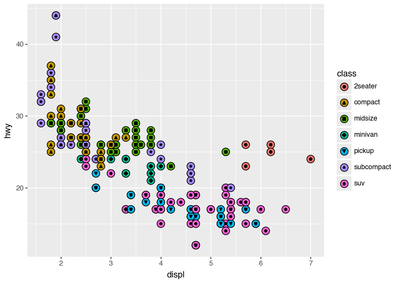
Geom functions determine how mapped data becomes visible marks. Layers are drawn in the order they are added.

(
    mpg.ggplot()
    .aes("displ", "hwy")
    .geom_point(aes(fill="class"), size=5)
    .geom_point(aes(shape="class"))
)

Individual Geoms

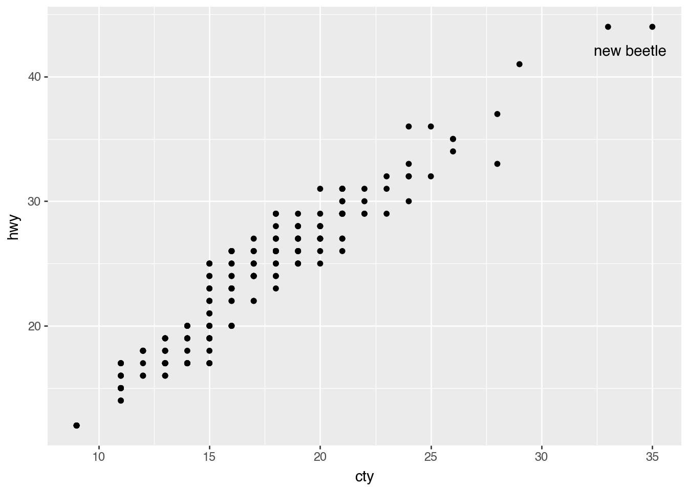
Scatterplot With Text

highest_mpg = mpg.filter(
    pl.col("hwy") == pl.col("hwy").max(),
    pl.col("cty") == pl.col("cty").max(),
)

(
    mpg.ggplot()
    .aes("cty", "hwy")
    .geom_point()
    .geom_text(
        aes(label="model"),
        nudge_y=-2,
        nudge_x=-1,
        data=highest_mpg,
    )
)

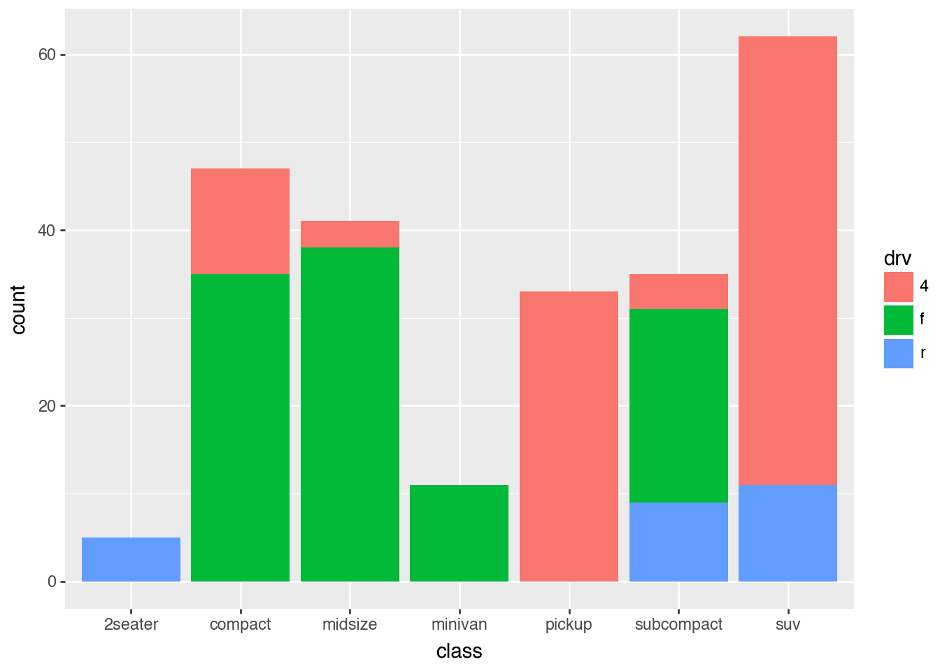
Barchart on Counts

counts = mpg.group_by("class", "drv").len().rename({"len": "count"})

(
    counts.ggplot()
    .aes("class", "count", fill="drv")
    .geom_col()
)

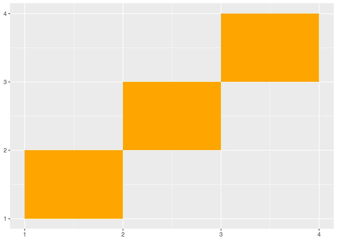
Rectangles

rectangles = pl.DataFrame(
    {
        "xmin": [1, 2, 3],
        "ymin": [1, 2, 3],
        "xmax": [2, 3, 4],
        "ymax": [2, 3, 4],
    }
)

(
    rectangles.ggplot()
    .aes(xmin="xmin", ymin="ymin", xmax="xmax", ymax="ymax")
    .geom_rect(fill="orange")
)

Collective Geoms for Distributions

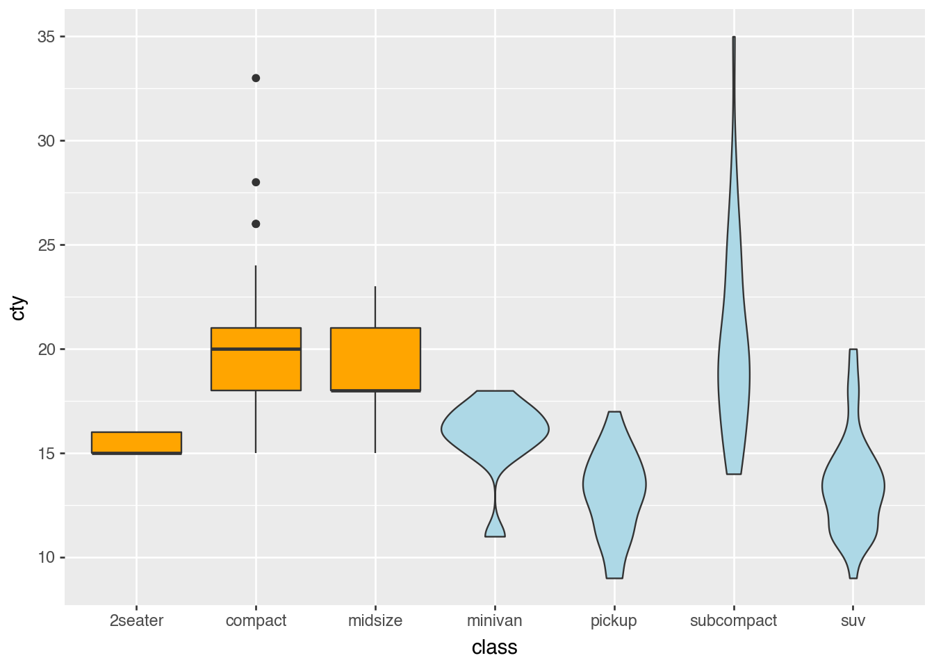
Boxplots and Violins

selected_classes = ["2seater", "compact", "midsize"]
mpg_box = mpg.filter(pl.col("class").is_in(selected_classes))
mpg_violin = mpg.filter(~pl.col("class").is_in(selected_classes))

(
    ggplot()
    .aes("class", "cty")
    .geom_boxplot(data=mpg_box, fill="orange")
    .geom_violin(data=mpg_violin, fill="lightblue")
)

/Users/igow/git/plotnine/plotnine/stats/stat.py:320: UserWarning: 
The following aesthetics were dropped during processing: ['y'].
plotnine could not infer the correct grouping.
Did you forget to specify a `group` aesthetic or to convert a numerical variable into a categorial?

Histograms and Densities

(
    mpg.ggplot()
    .aes("cty")
    .geom_histogram()
)

/Users/igow/git/plotnine/plotnine/stats/stat_bin.py:111: PlotnineWarning: 'stat_bin()' using 'bins = 17'. Pick better value with 'binwidth'.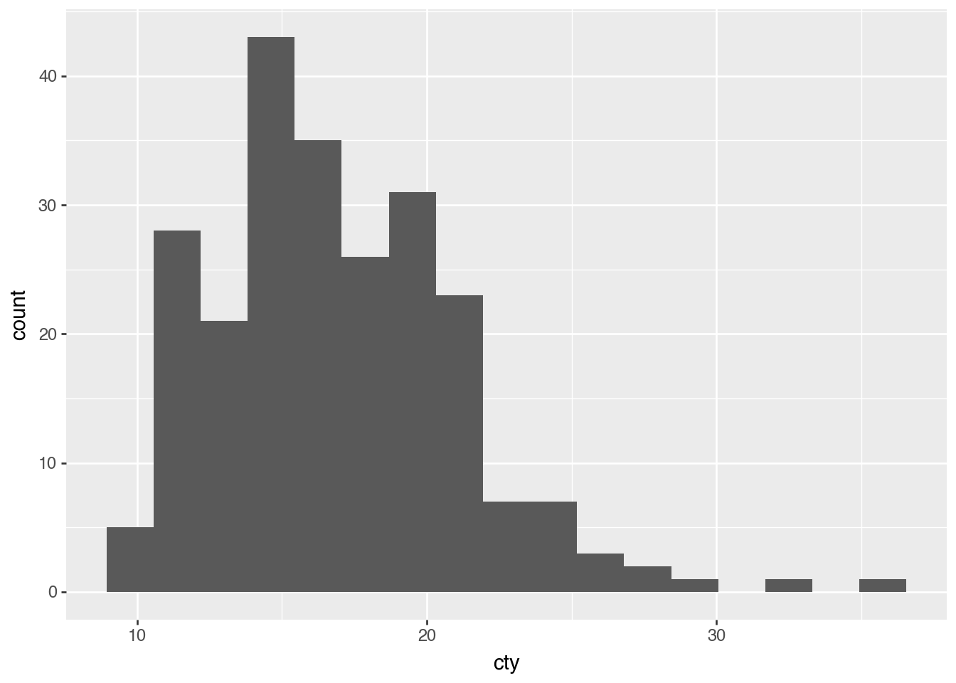

(
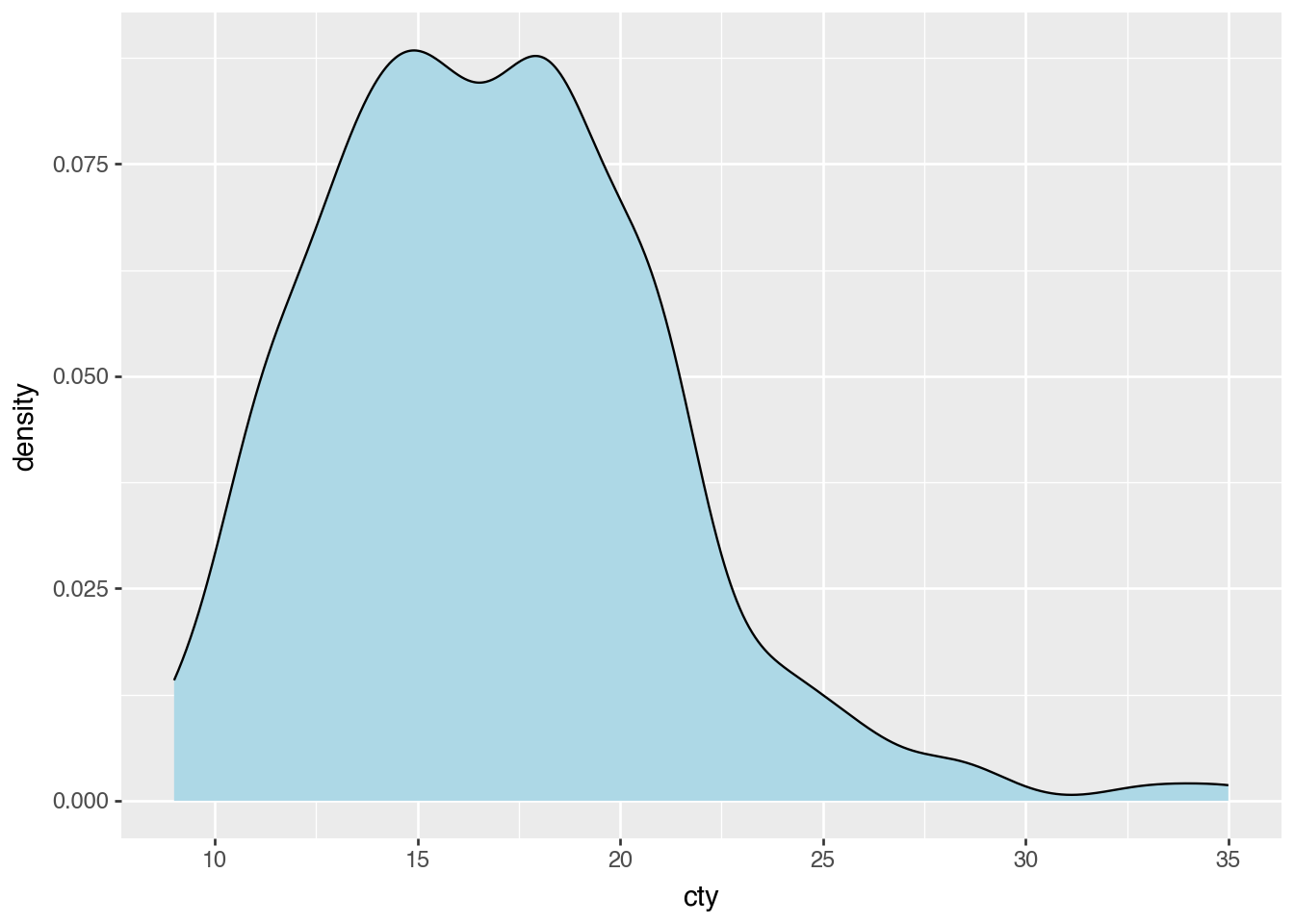
    mpg.ggplot()
    .aes("cty")
    .geom_density(fill="lightblue")
)

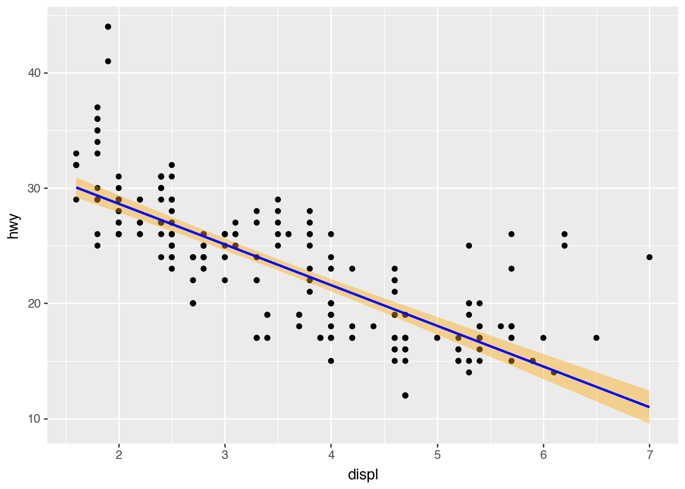
Smoothing

(
    mpg.ggplot()
    .aes("displ", "hwy")
    .geom_point()
    .geom_smooth(method="lm", color="blue", fill="orange")
)

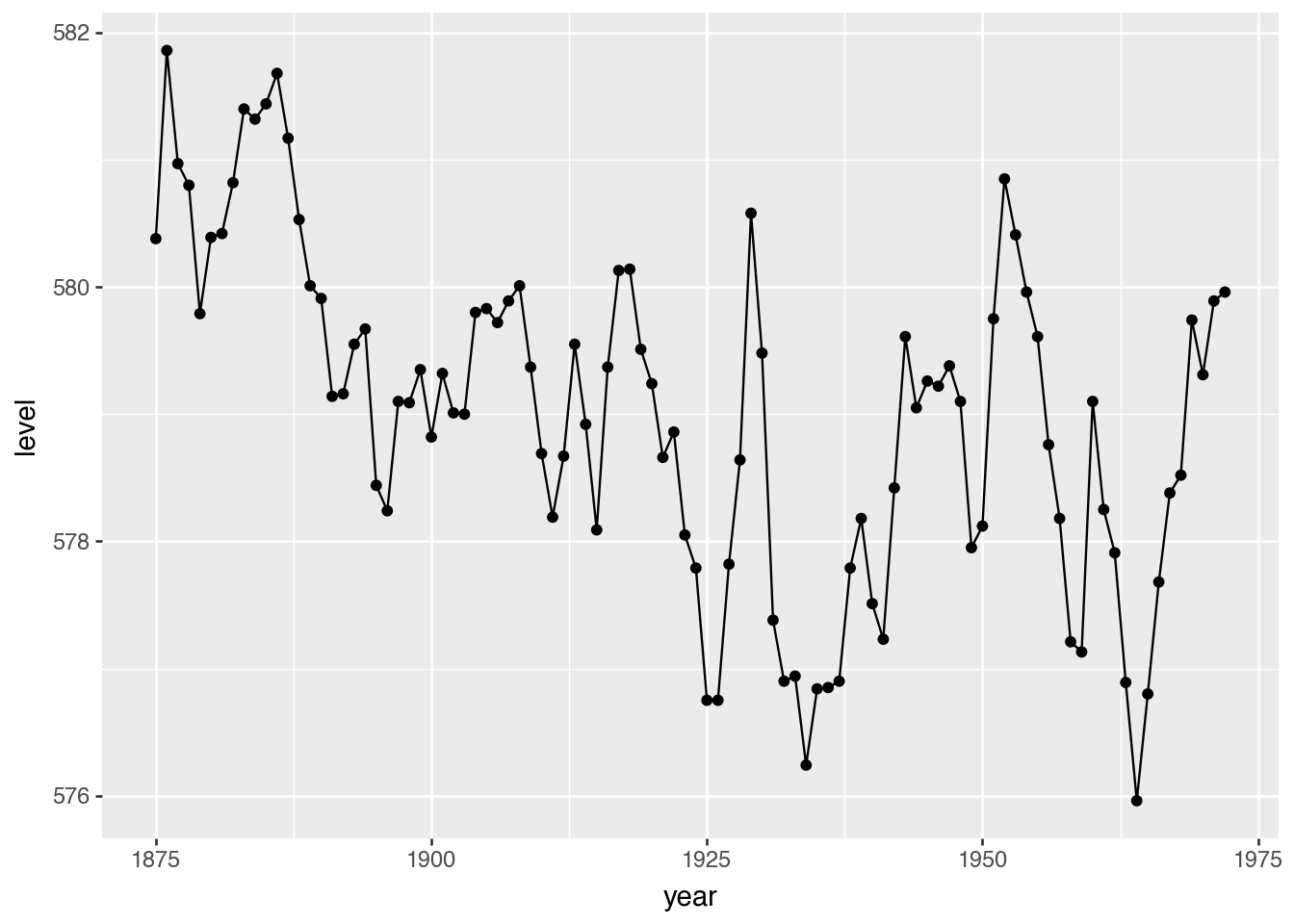
Collective Geoms for Lines and Fills

(
    huron.ggplot()
    .aes("year", "level")
    .geom_line()
    .geom_point()
)

(
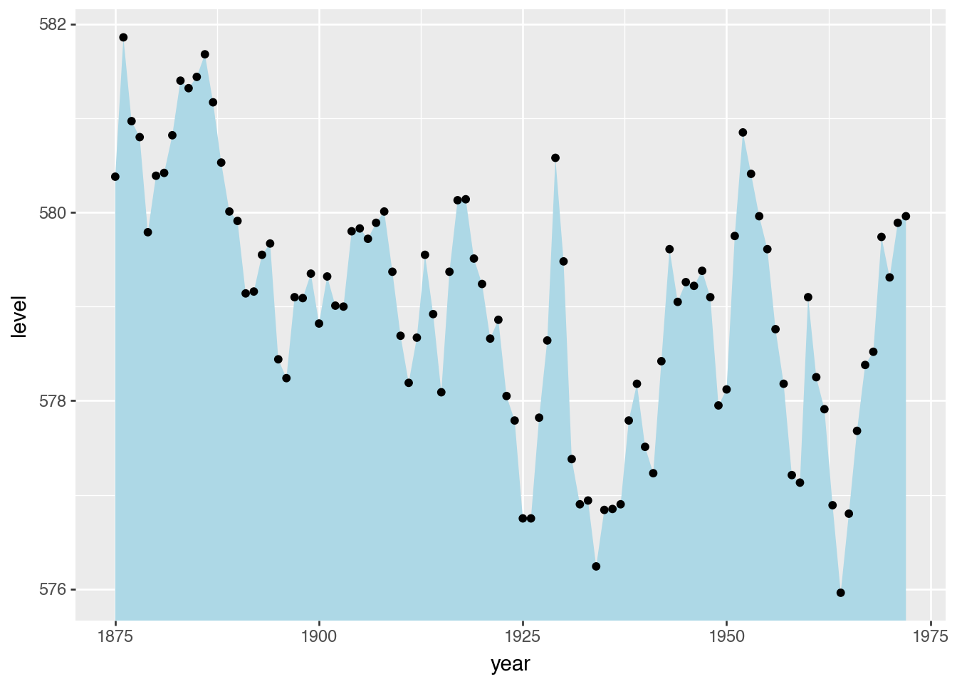
    huron.ggplot()
    .aes("year", "level")
    .geom_ribbon(aes(ymax="level"), ymin=0, fill="lightblue")
    .geom_point()
)

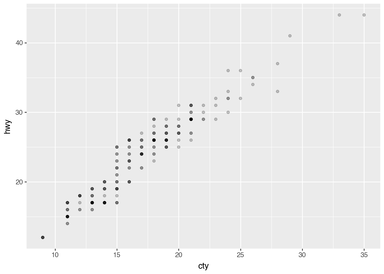
Position Adjustments

Jitter With Random Noise

(
    mpg.ggplot()
    .aes("cty", "hwy")
    .geom_point(alpha=0.2)
)

(
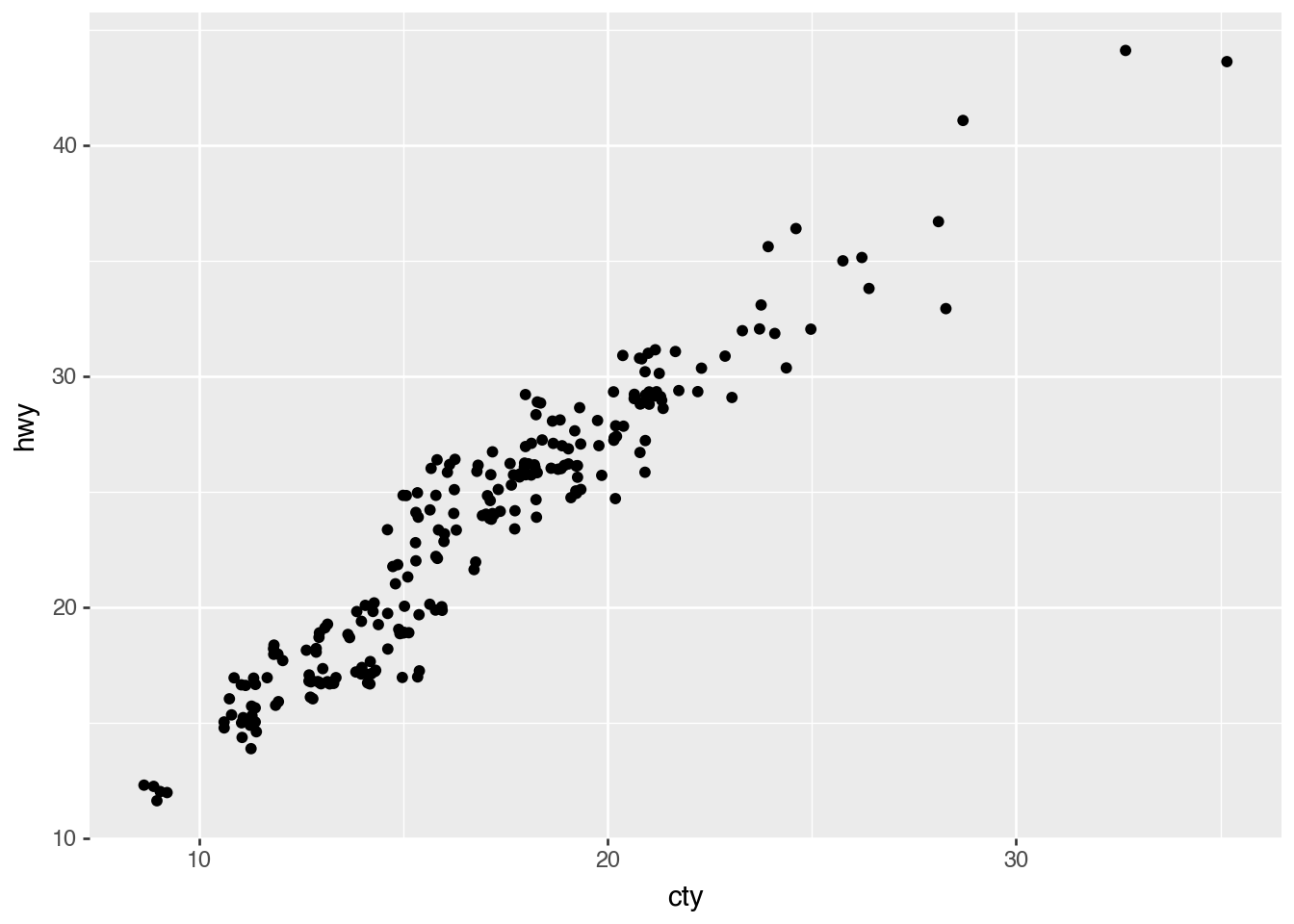
    mpg.ggplot()
    .aes("cty", "hwy")
    .geom_point(position=p9.position_jitter())
)

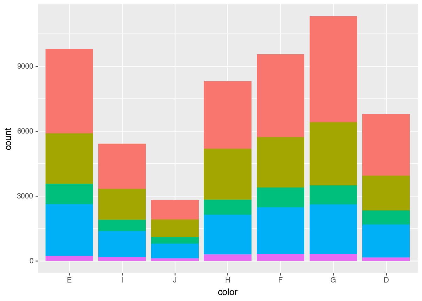
Dodge and Fill for Bars

(
    diamonds.ggplot()
    .aes("color", fill="cut")
    .add_theme(legend_position="none")
    .geom_bar()
)

(
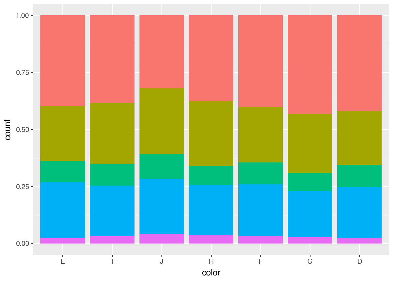
    diamonds.ggplot()
    .aes("color", fill="cut")
    .add_theme(legend_position="none")
    .geom_bar(position=p9.position_fill())
)

(
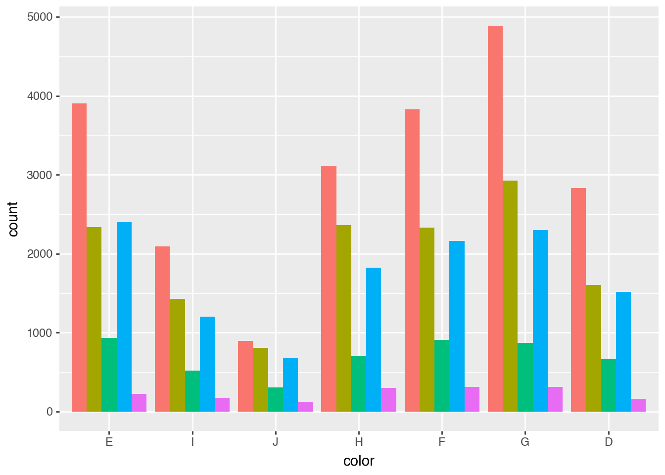
    diamonds.ggplot()
    .aes("color", fill="cut")
    .add_theme(legend_position="none")
    .geom_bar(position=p9.position_dodge())
)

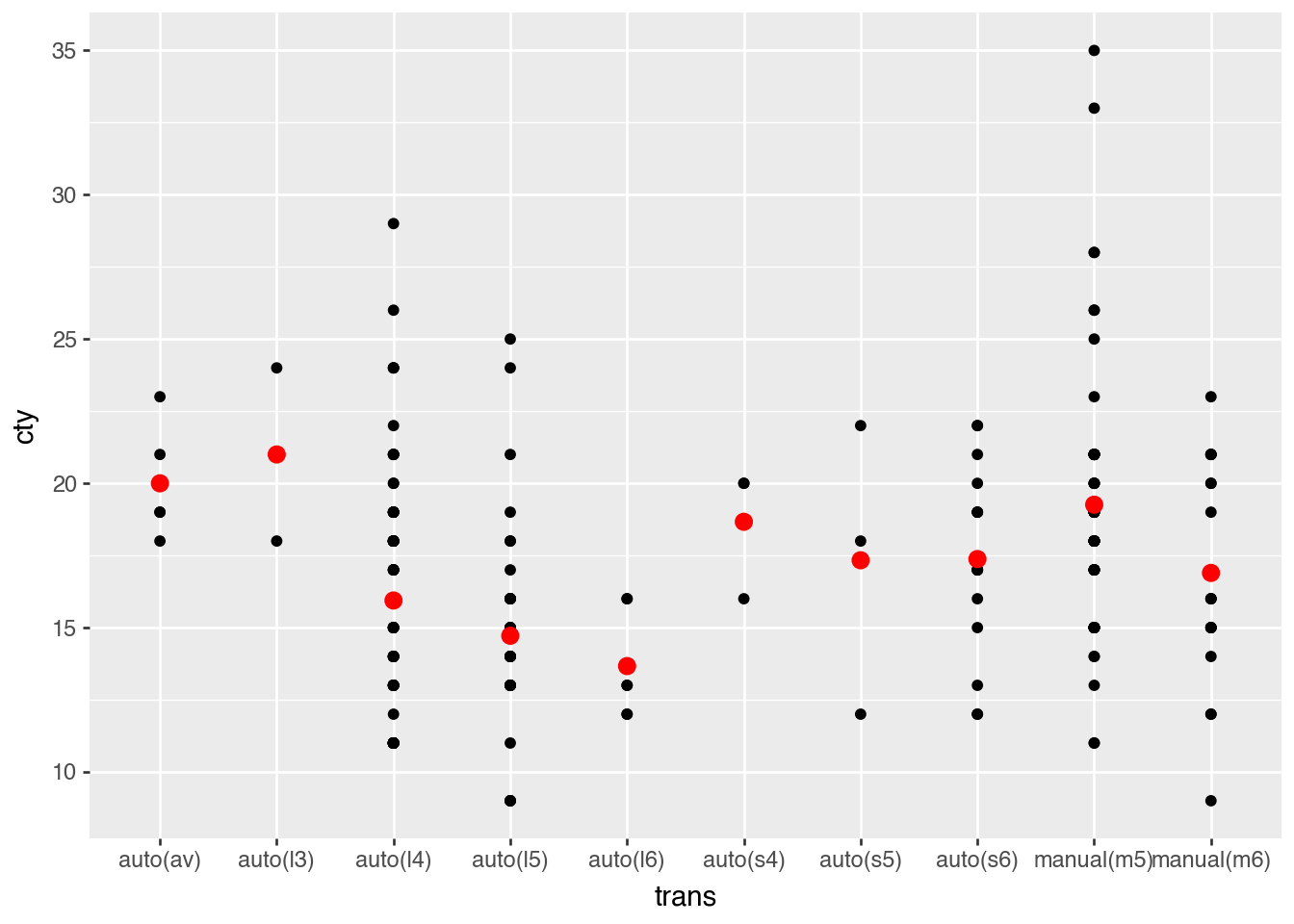
Statistical Transformations

(
    mpg.ggplot()
    .aes("trans", "cty")
    .geom_point()
    .geom_point(
        aes(group="trans"),
        color="red",
        size=3,
        stat="summary",
        fun_y=lambda x: x.mean(),
    )
)

mean_mpg = mpg.group_by("trans").agg(pl.col("cty").mean())
mean_mpg

shape: (10, 2)

trans	cty
str	f64
"auto(s4)"	18.666667
"auto(l4)"	15.939759
"auto(l3)"	21.0
"auto(l5)"	14.717949
"auto(s6)"	17.375
"manual(m6)"	16.894737
"manual(m5)"	19.258621
"auto(l6)"	13.666667
"auto(av)"	20.0
"auto(s5)"	17.333333

(
    mpg.ggplot()
    .aes("trans", "cty")
    .geom_point()
    .geom_point(data=mean_mpg, color="red", size=3)
)