import polars as pl
import plotnine_polars
from mizani.labels import label_comma
from plotnine import element_line, element_rect, element_textCiti Bike Trips Per Borough
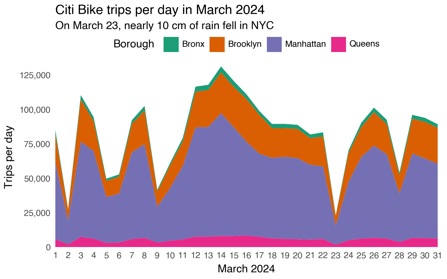
This page recreates the final plot shown just before the Load section in chapter 1 of Python Polars: The Definitive Guide, using plotnine_polars.
To keep the example focused on plotting, it uses a compact pre-aggregated table with daily trip counts by borough for March 2024.
Read the data
trips_per_day = (
    pl.read_csv(
        "../data/citi-bike-trips-per-day.csv",
        try_parse_dates=True,
    )
    .with_columns(
        pl.col("borough_start").cast(
            pl.Enum(["Bronx", "Brooklyn", "Manhattan", "Queens"])
        )
    )
)

trips_per_day
shape: (124, 3)
| borough_start | datetime_start | num_trips |
|---|---|---|
| enum | datetime[μs] | i64 |
| "Bronx" | 2024-03-01 00:00:00 | 2748 |
| "Brooklyn" | 2024-03-01 00:00:00 | 20068 |
| "Manhattan" | 2024-03-01 00:00:00 | 56434 |
| "Queens" | 2024-03-01 00:00:00 | 5728 |
| "Bronx" | 2024-03-02 00:00:00 | 1010 |
| … | … | … |
| "Queens" | 2024-03-30 00:00:00 | 6583 |
| "Bronx" | 2024-03-31 00:00:00 | 2724 |
| "Brooklyn" | 2024-03-31 00:00:00 | 25940 |
| "Manhattan" | 2024-03-31 00:00:00 | 54440 |
| "Queens" | 2024-03-31 00:00:00 | 6237 |
Plot
(
    trips_per_day.ggplot()
    .aes(x="datetime_start", y="num_trips", fill="borough_start")
    .geom_area()
    .scale_fill_brewer(type="qual", palette=2)
    .scale_x_datetime(date_labels="%-d", date_breaks="1 day", expand=(0, 0))
    .scale_y_continuous(labels=label_comma(), expand=(0, 0))
    .labs(
        x="March 2024",
        fill="Borough",
        y="Trips per day",
        title="Citi Bike trips per day in March 2024",
        subtitle="On March 23, nearly 10 cm of rain fell in NYC",
    )
    .theme_tufte(base_size=14)
    .add_theme(
        axis_ticks_major=element_line(color="white"),
        figure_size=(8, 5),
        legend_position="top",
        plot_background=element_rect(fill="white", color="white"),
        plot_caption=element_text(style="italic"),
        plot_title=element_text(ha="left"),
    )
)