6  Univariate Portfolio Sorts

library(tidyverse)
library(DBI)
library(scales)
library(lmtest)
library(sandwich)

6.1 Data Preparation

tidy_finance <- dbConnect(
  duckdb::duckdb(),
  "data/tidy_finance.duckdb",
  read_only = TRUE)

There are three tables used for this chapter. I defer the select() used with crsp_monthly in the book, as I find it more elegant to have a code chunk that just links to the database tables.

crsp_monthly <- tbl(tidy_finance, "crsp_monthly") 
factors_ff_monthly <- tbl(tidy_finance, "factors_ff_monthly")
beta <- tbl(tidy_finance, "beta_alt")

6.2 Sorting by Market Beta

beta_lag <- 
  beta |>
  mutate(month = month + months(1)) |>
  select(permno, month, beta_lag = beta_monthly) |>
  filter(!is.na(beta_lag))

data_for_sorts <- 
  crsp_monthly |>
  select(permno, month, ret_excess, mktcap_lag) |>
  inner_join(beta_lag, by = c("permno", "month"))

breakpoints <-
  data_for_sorts |>
  group_by(month) |>
  summarize(breakpoint = median(beta_lag, na.rm = TRUE),
            .groups = "drop")

beta_portfolios <- 
  data_for_sorts |>
  inner_join(breakpoints, by = "month") |>
  mutate(
    portfolio = case_when(
      beta_lag <= breakpoint ~ "low",
      beta_lag > breakpoint ~ "high")) |>
  filter(!is.na(ret_excess)) |>
  group_by(month, portfolio) |>
  summarize(ret = sum(ret_excess * mktcap_lag, na.rm = TRUE)/
              sum(mktcap_lag, na.rm = TRUE), 
            .groups = "drop")

6.3 Performance Evaluation

beta_longshort <- 
  beta_portfolios |>
  pivot_wider(id_cols = month, names_from = portfolio, values_from = ret) |>
  mutate(long_short = high - low) |>
  collect()

model_fit <- lm(long_short ~ 1, data = beta_longshort)
coeftest(model_fit, vcov = NeweyWest)

t test of coefficients:

              Estimate Std. Error t value Pr(>|t|)
(Intercept) 0.00013932 0.00107096  0.1301   0.8965

6.4 Functional Programming for Portfolio Sorts

Using the ntile() function, the assign_portfolio() function can be reduced to a one-liner. As such there is no reason to have a function, but I have retained this to illustrate the use of the curly-curly operator as shown in the book.

assign_portfolio <- function(data, var, n_portfolios) {
  mutate(data, portfolio = ntile({{ var }}, n_portfolios))
}

Using a “data-frame-in-data-frame-out” function results in tidier code. Because the data are still in the database, we use our home-brewed alternative to weighted.mean() and defer the conversion of portfolio to a factor until we collect() the data below.

beta_portfolios <- 
  data_for_sorts |>
  group_by(month) |>
  assign_portfolio(var = beta_lag, 10) |>
  group_by(portfolio, month) |>
  summarize(ret = sum(ret_excess * mktcap_lag, na.rm = TRUE)/
                    sum(mktcap_lag, na.rm = TRUE), 
            .groups = "drop")

6.5 More Performance Evaluation

Unlike the book, I use the coef() function here for a small amount of convenience.

beta_portfolios_summary <- 
  beta_portfolios |>
  left_join(factors_ff_monthly, by = "month") |>
  group_by(portfolio) |>
  collect() %>%
  mutate(portfolio = as.factor(portfolio)) |>
  summarize(
    alpha = coef(lm(ret ~ 1 + mkt_excess))[1],
    beta = coef(lm(ret ~ 1 + mkt_excess))[2],
    ret = mean(ret)
  )

beta_portfolios_summary |>
  ggplot(aes(x = portfolio, y = alpha, fill = portfolio)) +
  geom_bar(stat = "identity") +
  labs(
    title = "CAPM alphas of beta-sorted portfolios",
    x = "Portfolio",
    y = "CAPM alpha",
    fill = "Portfolio"
  ) +
  scale_y_continuous(labels = percent) +
  theme(legend.position = "None")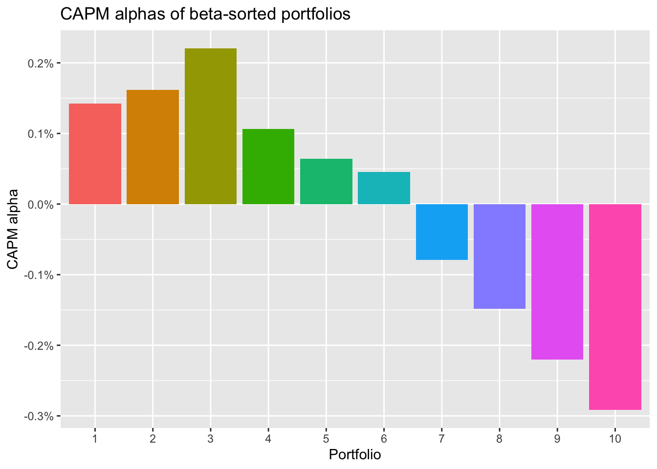

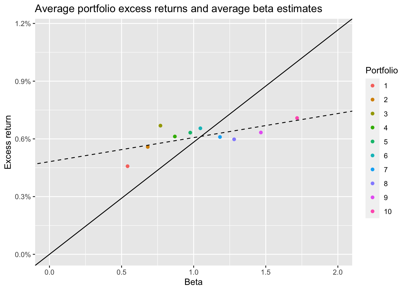
Figure 6.1: Portfolios are sorted into deciles each month based on their estimated CAPM beta. The bar charts indicate the CAPM alpha of the resulting portfolio returns during the entire CRSP period.

6.6 The Security Market Line and Beta Portfolios

Again I use the coef() function and I also extract the calculation stored in mean_mkt_excess upfront.

sml_capm <- coef(lm(ret ~ 1 + beta, data = beta_portfolios_summary))

mean_mkt_excess <- 
  factors_ff_monthly |>
  summarize(mean(mkt_excess, na.rm = TRUE)) |>
  pull()

beta_portfolios_summary |>
  filter(!is.na(ret), !is.na(beta)) |>
  ggplot(aes(
    x = beta, 
    y = ret, 
    color = portfolio
  )) +
  geom_point() +
  geom_abline(
    intercept = 0,
    slope = mean_mkt_excess,
    linetype = "solid"
  ) +
  geom_abline(
    intercept = sml_capm[1],
    slope = sml_capm[2],
    linetype = "dashed"
  ) +
  scale_y_continuous(
    labels = percent,
    limit = c(0, mean_mkt_excess * 2)
  ) +
  scale_x_continuous(limits = c(0, 2)) +
  labs(
    x = "Beta", y = "Excess return", color = "Portfolio",
    title = "Average portfolio excess returns and average beta estimates"
  )

Figure 6.2: Excess returns are computed as CAPM alphas of the beta-sorted portfolios. The horizontal axis indicates the CAPM beta of the resulting beta-sorted portfolio return time series. The dashed line indicates the slope coefficient of a linear regression of excess returns on portfolio betas.

The ungroup() shown in the book is not needed (because we used .groups = "drop") in the previous step.

beta_longshort <- 
  beta_portfolios |>
  mutate(portfolio = case_when(
    portfolio == max(as.numeric(portfolio)) ~ "high",
    portfolio == min(as.numeric(portfolio)) ~ "low"
  )) |>
  filter(portfolio %in% c("low", "high")) |>
  pivot_wider(id_cols = month, names_from = portfolio, values_from = ret) |>
  mutate(long_short = high - low) |>
  left_join(factors_ff_monthly, by = "month") %>%
  collect()

Warning: Missing values are always removed in SQL aggregation functions.
Use `na.rm = TRUE` to silence this warning
This warning is displayed once every 8 hours.

coeftest(lm(long_short ~ 1, data = beta_longshort),
         vcov = NeweyWest)

t test of coefficients:

             Estimate Std. Error t value Pr(>|t|)
(Intercept) 0.0025049  0.0027858  0.8992   0.3689

coeftest(lm(long_short ~ 1 + mkt_excess, data = beta_longshort),
         vcov = NeweyWest)

t test of coefficients:

              Estimate Std. Error t value Pr(>|t|)    
(Intercept) -0.0043407  0.0021566 -2.0128  0.04453 *  
mkt_excess   1.1755556  0.0679566 17.2986  < 2e-16 ***
---
Signif. codes:  0 '***' 0.001 '**' 0.01 '*' 0.05 '.' 0.1 ' ' 1

We have already applied collect() to beta_longshort, so we can use R functions here. If beta_longshort were a remote data frame, not that dbplyr does not translate prod() for us, but we could use the product() aggregate from DuckDB.

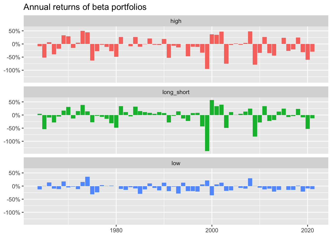
beta_longshort |>
  group_by(year = year(month)) |>
  summarize(
    low = prod(1 + low),
    high = prod(1 + high),
    long_short = prod(1 + long_short)
  ) |>
  pivot_longer(cols = -year) |>
  ggplot(aes(x = year, y = 1 - value, fill = name)) +
  geom_col(position = "dodge") +
  facet_wrap(~name, ncol = 1) +
  theme(legend.position = "none") +
  scale_y_continuous(labels = percent) +
  labs(
    title = "Annual returns of beta portfolios",
    x = NULL, y = NULL
  )

dbDisconnect(tidy_finance, shutdown = TRUE)