library(tidyverse)
library(DBI)
library(scales)
library(sandwich)
library(lmtest)
library(dbplyr)
library(rlang)7 Size Sorts and p-Hacking
We do not need the furr package for the dbplyr version of the code, but we do load the dbplyr package so that we can access the window_order() function below.
library(tidyverse)
library(DBI)
library(scales)
library(sandwich)
library(lmtest)
library(furrr)
library(rlang)
7.1 Data Preparation
tidy_finance <- dbConnect(
  duckdb::duckdb(),
  "data/tidy_finance.duckdb",
  read_only = TRUE)

crsp_monthly <-
  tbl(tidy_finance, "crsp_monthly")


factors_ff_monthly <-
  tbl(tidy_finance, "factors_ff_monthly")
tidy_finance <- dbConnect(
duckdb::duckdb(),
"data/tidy_finance.duckdb",
read_only = TRUE)
crsp_monthly <-
tbl(tidy_finance, "crsp_monthly") |>
collect()
factors_ff_monthly <-
tbl(tidy_finance, "factors_ff_monthly") |>
collect() 7.2 Size Distribution
In the following code, we need to make a few tweaks in translating it to dbplyr.
First, we want to extract the calculations of quantiles by month into a separate query. These calculations are grouped aggregates, so should happen inside a group_by()/summarize() query in SQL. We also include the calculation of total_market_cap in this query.
Second, I simplify the creation of the quantile indicators (e.g., top01). There is no need to write if_else(condition == TRUE, 1, 0) when condition will effectively yield the same result. This means that we do not need to write mktcap[top01 == 1], but can use mktcap[top01].
Third, the original approach has calculations such as sum(mktcap[top01 == 1]) / total_market_cap inside a summarize() call. However, SQL implementations are normally strict in requiring variables to appear either inside an aggregate function (e.g., sum()) or as part of the grouping (group_by or GROUP BY). In the original calculation is outside the sum() aggregate and not part of the grouping set (we have group_by(month)).
Fourth, because we want to use factors for the plot, we need to collect() before constructing the factor.
Otherwise the two approaches are the same.
monthly_quantiles <-
  crsp_monthly |>
  group_by(month) |>
  summarize(
    total_market_cap = sum(mktcap, na.rm = TRUE),
    q_top01 = quantile(mktcap, 0.99),
    q_top05 = quantile(mktcap, 0.95),
    q_top10 = quantile(mktcap, 0.90),
    q_top25 = quantile(mktcap, 0.75),
    .groups = "drop")

crsp_monthly |>
  inner_join(monthly_quantiles, by = "month") |>
  mutate(
    top01 = mktcap >= q_top01,
    top05 = mktcap >= q_top05,
    top10 = mktcap >= q_top10,
    top25 = mktcap >= q_top25,
    .groups = "drop") |>
  group_by(month) |>
  summarize(
    `Largest 1% of stocks` = sum(mktcap[top01]/total_market_cap),
    `Largest 5% of stocks` = sum(mktcap[top05]/total_market_cap),
    `Largest 10% of stocks` = sum(mktcap[top10]/total_market_cap),
    `Largest 25% of stocks` = sum(mktcap[top25]/total_market_cap),
    .groups = "drop") |>
  pivot_longer(cols = -month) |>
  collect() |>
  mutate(name = factor(name, levels = c(
    "Largest 1% of stocks", "Largest 5% of stocks",
    "Largest 10% of stocks", "Largest 25% of stocks"
  ))) |>
  ggplot(aes(
    x = month,
    y = value,
    color = name,
    linetype = name)) +
  geom_line() +
  scale_y_continuous(labels = percent, limits = c(0, 1)) +
  labs(
    x = NULL, y = NULL, color = NULL, linetype = NULL,
    title = "Percentage of total market capitalization in largest stocks")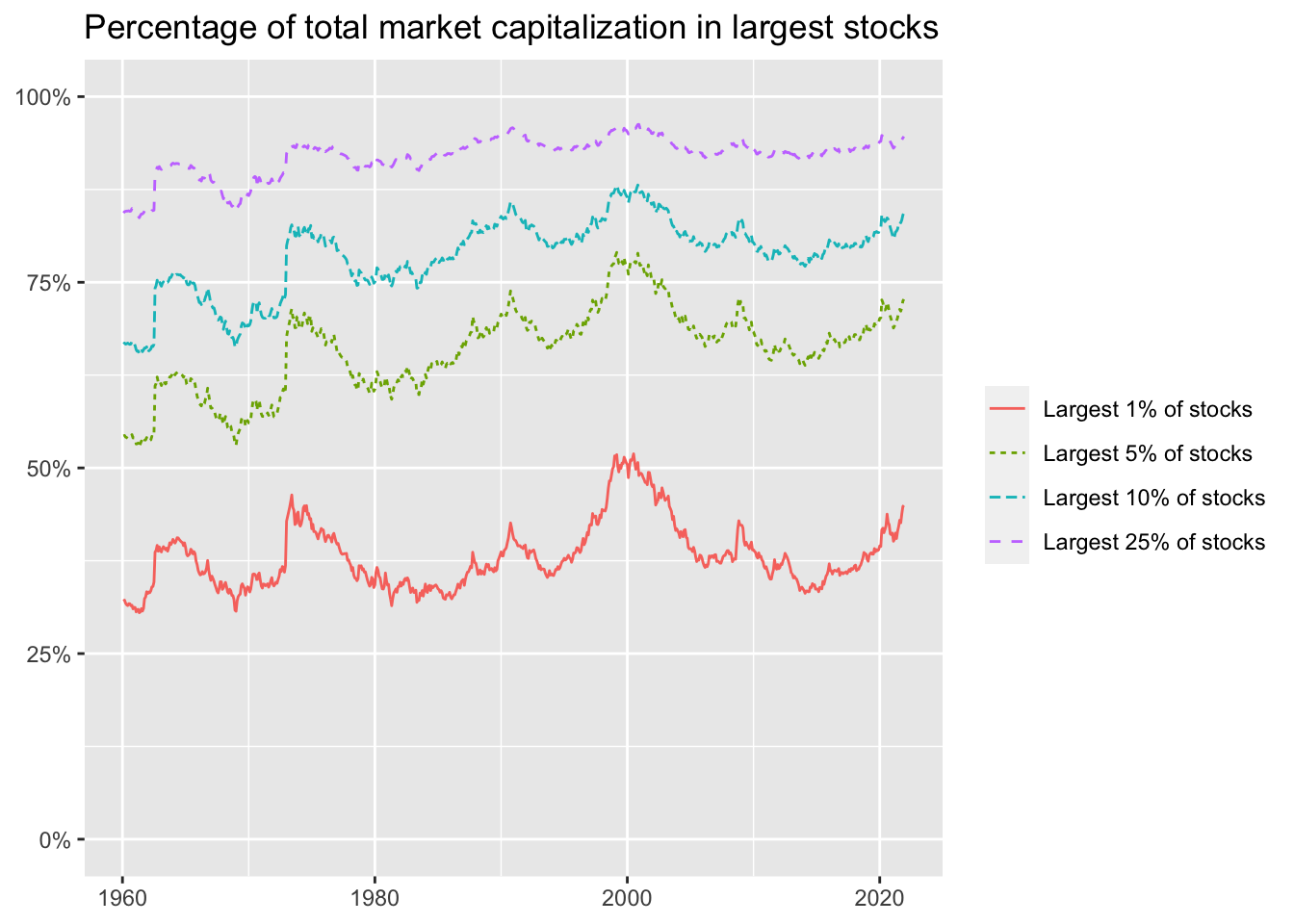
crsp_monthly |>
  group_by(month) |>
  mutate(
    top01 = if_else(mktcap >= quantile(mktcap, 0.99), 1, 0),
    top05 = if_else(mktcap >= quantile(mktcap, 0.95), 1, 0),
    top10 = if_else(mktcap >= quantile(mktcap, 0.90), 1, 0),
    top25 = if_else(mktcap >= quantile(mktcap, 0.75), 1, 0)
  ) |>
  summarize(
    total_market_cap =  sum(mktcap),
    `Largest 1% of stocks` = sum(mktcap[top01 == 1]) / total_market_cap,
    `Largest 5% of stocks` = sum(mktcap[top05 == 1]) / total_market_cap,
    `Largest 10% of stocks` = sum(mktcap[top10 == 1]) / total_market_cap,
    `Largest 25% of stocks` = sum(mktcap[top25 == 1]) / total_market_cap,
    .groups = "drop"
  ) |>
  select(-total_market_cap) |>
  pivot_longer(cols = -month) |>
  mutate(name = factor(name, levels = c(
    "Largest 1% of stocks", "Largest 5% of stocks",
    "Largest 10% of stocks", "Largest 25% of stocks"
  ))) |>
  ggplot(aes(
    x = month,
    y = value,
    color = name,
    linetype = name)) +
  geom_line() +
  scale_y_continuous(labels = percent, limits = c(0, 1)) +
  labs(
    x = NULL, y = NULL, color = NULL, linetype = NULL,
    title = "Percentage of total market capitalization in largest stocks"
  )
The next code chunk is the same.
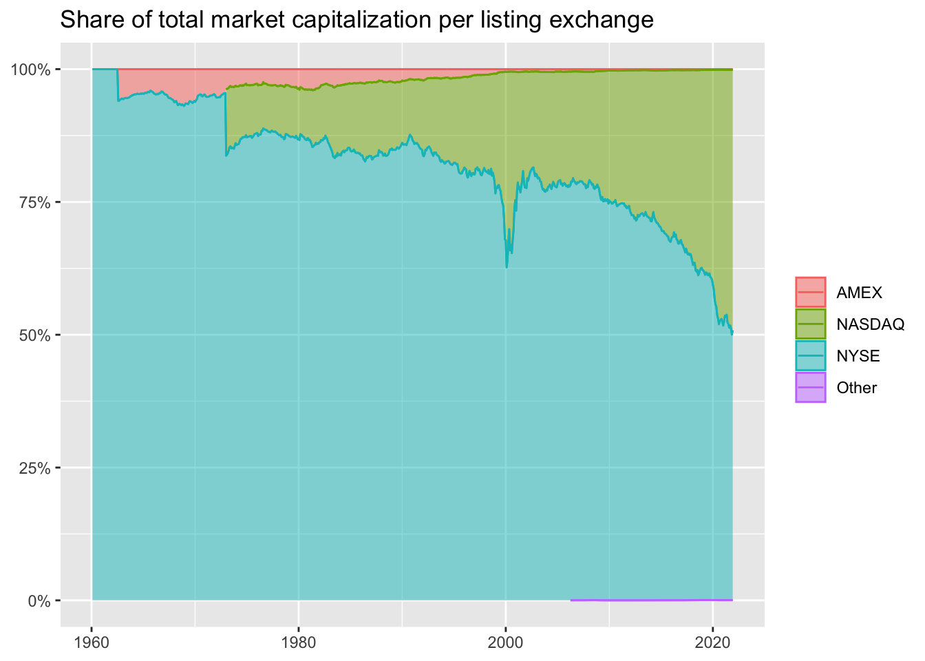
crsp_monthly |>
  group_by(month, exchange) |>
  summarize(mktcap = sum(mktcap),
            .groups = "drop_last") |>
  mutate(share = mktcap / sum(mktcap)) |>
  ggplot(aes(
    x = month,
    y = share,
    fill = exchange,
    color = exchange)) +
  geom_area(
    position = "stack",
    stat = "identity",
    alpha = 0.5
  ) +
  geom_line(position = "stack") +
  scale_y_continuous(labels = percent) +
  labs(
    x = NULL, y = NULL, fill = NULL, color = NULL,
    title = "Share of total market capitalization per listing exchange"
  )
create_summary <- function(data, column_name) {
  data |>
    select(value = {{ column_name }}) |>
    summarize(
      mean = mean(value),
      sd = sd(value),
      min = min(value),
      q05 = quantile(value, 0.05),
      q50 = quantile(value, 0.50),
      q95 = quantile(value, 0.95),
      max = max(value),
      n = n()
    )
}

crsp_monthly |>
  filter(month == max(month)) |>
  group_by(exchange) |>
  create_summary(mktcap) |>
  arrange(exchange) |>
  union_all(crsp_monthly |>
            filter(month == max(month)) |>
            create_summary(mktcap) |>
            mutate(exchange = "Overall")) |>
  collect()
Adding missing grouping variables: `exchange`| exchange | mean | sd | min | q05 | q50 | q95 | max | n |
|---|---|---|---|---|---|---|---|---|
| AMEX | 414.7685 | 2180.64 | 7.56557 | 12.55276 | 75.83695 | 1218.314 | 25718.89 | 145 |
| NASDAQ | 8650.8801 | 90037.57 | 7.00553 | 29.30835 | 429.09850 | 18780.584 | 2902368.14 | 2779 |
| NYSE | 17857.7021 | 48618.73 | 23.91300 | 194.98000 | 3433.58503 | 80748.492 | 472941.07 | 1395 |
| Other | 13906.2461 | NA | 13906.24613 | 13906.24613 | 13906.24613 | 13906.246 | 13906.25 | 1 |
| Overall | 11348.6893 | 77458.26 | 7.00553 | 34.31473 | 795.59922 | 40647.106 | 2902368.14 | 4320 |
create_summary <- function(data, column_name) {
  data |>
    select(value = {{ column_name }}) |>
    summarize(
      mean = mean(value),
      sd = sd(value),
      min = min(value),
      q05 = quantile(value, 0.05),
      q50 = quantile(value, 0.50),
      q95 = quantile(value, 0.95),
      max = max(value),
      n = n()
    )
}

crsp_monthly |>
  filter(month == max(month)) |>
  group_by(exchange) |>
  create_summary(mktcap) |>
  add_row(crsp_monthly |>
            filter(month == max(month)) |>
            create_summary(mktcap) |>
mutate(exchange = "Overall"))get_breaks <- function(data, n_portfolios, exchanges) {
ports <- 0:n_portfolios
ports_sql <- sql(paste0("[", paste(ports, collapse = ", "), "]"))
breaks <- seq(0, 1, 1/n_portfolios)
breaks_sql <- sql(paste0("[", paste(breaks, collapse = ", "), "]"))
data |>
filter(exchange %in% exchanges) |>
summarize(portfolio = ports_sql,
breaks = quantile_cont(mktcap_lag, breaks_sql),
.groups = "keep") %>%
mutate(portfolio = unnest(portfolio),
breaks = unnest(breaks)) |>
group_by(month) |>
window_order(portfolio) |>
mutate(port_max = if_else(portfolio == n_portfolios, Inf, breaks),
port_min = if_else(portfolio == 1, -Inf, lag(breaks))) |>
filter(portfolio > 0) |>
select(month, portfolio, port_max, port_min) |>
ungroup() |>
compute()
}
assign_portfolio <- function(data, n_portfolios, exchanges) {
breaks <- get_breaks(data, n_portfolios, exchanges)
data |>
inner_join(breaks,
join_by(month,
mktcap_lag >= port_min,
mktcap_lag < port_max)) |>
select(-port_min, -port_max)
}assign_portfolio <- function(n_portfolios,
exchanges,
data) {
breakpoints <- data |>
filter(exchange %in% exchanges) |>
reframe(breakpoint = quantile(
mktcap_lag,
probs = seq(0, 1, length.out = n_portfolios + 1),
na.rm = TRUE
)) |>
pull(breakpoint) |>
as.numeric()
assigned_portfolios <- data |>
mutate(portfolio = findInterval(mktcap_lag,
breakpoints,
all.inside = TRUE
)) |>
pull(portfolio)
return(assigned_portfolios)
}Here I tweak the code so that the data argument comes first in compute_portfolio_returns(). This facilitates a pipe-based approach, which I use below in the dbplyr code.
With the dbplyr approach we have no weighted.mean() function to use. Instead, we calculate the weighted mean “by hand” and set weight = if_else(value_weighted, mktcap_lag, 1) (i.e., weight is mktcap_lag for value-weighted returns, but one otherwise).
compute_portfolio_returns <-
  function(data = crsp_monthly,
           n_portfolios = 10,
           exchanges = c("NYSE", "NASDAQ", "AMEX"),
           value_weighted = TRUE) {

  exchanges_str <- str_flatten(exchanges, ", ")

  data |>
    group_by(month) |>
    assign_portfolio(n_portfolios, exchanges) |>
    group_by(month, portfolio) |>
    filter(!is.na(ret), !is.na(mktcap_lag)) |>
    mutate(weight = if_else(value_weighted, mktcap_lag, 1)) |>
    summarize(
       ret = sum(ret_excess * weight, na.rm = TRUE)/
                    sum(weight, na.rm = TRUE),
      .groups = "drop") |>
    mutate(portfolio = case_when(portfolio == min(portfolio) ~ "min",
                                 portfolio == max(portfolio) ~ "max",
                                 TRUE ~ "other")) |>
    filter(portfolio %in% c("min", "max")) |>
    pivot_wider(names_from = portfolio, values_from = ret) |>
    mutate(size_premium = min - max) |>
    summarize(size_premium = mean(size_premium)) |>
    mutate(exchanges = exchanges_str) |>
    select(exchanges, size_premium) |>
    collect()
}
compute_portfolio_returns <-
function(data = crsp_monthly,
n_portfolios = 10,
exchanges = c("NYSE", "NASDAQ", "AMEX"),
value_weighted = TRUE) {
data |>
group_by(month) |>
mutate(portfolio = assign_portfolio(
n_portfolios = n_portfolios,
exchanges = exchanges,
data = pick(everything())
)) |>
group_by(month, portfolio) |>
summarize(
ret = if_else(value_weighted,
weighted.mean(ret_excess, mktcap_lag),
mean(ret_excess)
),
.groups = "drop_last"
) |>
summarize(size_premium = ret[portfolio == min(portfolio)] -
ret[portfolio == max(portfolio)]) |>
summarize(size_premium = mean(size_premium))
}ret_all <-
crsp_monthly |>
compute_portfolio_returns(n_portfolios = 2,
exchanges = c("NYSE", "NASDAQ", "AMEX"),
value_weighted = TRUE)
ret_nyse <-
crsp_monthly |>
compute_portfolio_returns(n_portfolios = 2,
exchanges = "NYSE",
value_weighted = TRUE)
bind_rows(ret_all, ret_nyse)| exchanges | size_premium |
|---|---|
| NYSE, NASDAQ, AMEX | 0.000975 |
| NYSE | 0.001664 |
ret_all <- compute_portfolio_returns(
  n_portfolios = 2,
  exchanges = c("NYSE", "NASDAQ", "AMEX"),
  value_weighted = TRUE,
  data = crsp_monthly
)

ret_nyse <- compute_portfolio_returns(
  n_portfolios = 2,
  exchanges = "NYSE",
  value_weighted = TRUE,
  data = crsp_monthly
)

tibble(
  Exchanges = c("NYSE, NASDAQ & AMEX", "NYSE"),
  Premium = as.numeric(c(ret_all, ret_nyse)) * 100
)
The code for p_hacking_setup is common across the two approaches.
p_hacking_setup <-
  expand_grid(
    n_portfolios = c(2, 5, 10),
    exchanges = list("NYSE", c("NYSE", "NASDAQ", "AMEX")),
    value_weighted = c(TRUE, FALSE),
    data = parse_exprs(
     'crsp_monthly;
      crsp_monthly |> filter(industry != "Finance");
      crsp_monthly |> filter(month < "1990-06-01");
      crsp_monthly |> filter(month >="1990-06-01")'))
Because DuckDB will use multiple cores without explicit instructions, I don’t need to set up multisession with the dbplyr approach.
p_hacking_setup <-
  p_hacking_setup |>
  mutate(size_premium =
           pmap(.l = list(data, n_portfolios, exchanges, value_weighted),
                .f = ~ compute_portfolio_returns(
                  data = eval_tidy(..1),
                  n_portfolios = ..2,
                  exchanges = ..3,
value_weighted = ..4)))plan(multisession, workers = availableCores())
p_hacking_setup <- p_hacking_setup |>
mutate(size_premium = future_pmap(
.l = list(
n_portfolios,
exchanges,
value_weighted,
data
),
.f = ~ compute_portfolio_returns(
n_portfolios = ..1,
exchanges = ..2,
value_weighted = ..3,
data = eval_tidy(..4)
)
))p_hacking_results <-
p_hacking_setup |>
select(-exchanges) |>
mutate(data = map_chr(data, deparse)) |>
unnest(size_premium) |>
arrange(desc(size_premium)) |>
filter(!is.na(size_premium))
p_hacking_results| n_portfolios | value_weighted | data | exchanges | size_premium |
|---|---|---|---|---|
| 10 | FALSE | filter(crsp_monthly, month >= “1990-06-01”) | NYSE, NASDAQ, AMEX | 0.0186423 |
| 10 | FALSE | filter(crsp_monthly, industry != “Finance”) | NYSE, NASDAQ, AMEX | 0.0182132 |
| 10 | FALSE | crsp_monthly | NYSE, NASDAQ, AMEX | 0.0163249 |
| 10 | FALSE | filter(crsp_monthly, month < “1990-06-01”) | NYSE, NASDAQ, AMEX | 0.0139120 |
| 10 | TRUE | filter(crsp_monthly, industry != “Finance”) | NYSE, NASDAQ, AMEX | 0.0115089 |
| 10 | TRUE | filter(crsp_monthly, month < “1990-06-01”) | NYSE, NASDAQ, AMEX | 0.0109079 |
| 10 | TRUE | crsp_monthly | NYSE, NASDAQ, AMEX | 0.0102892 |
| 10 | TRUE | filter(crsp_monthly, month >= “1990-06-01”) | NYSE, NASDAQ, AMEX | 0.0096950 |
| 5 | FALSE | filter(crsp_monthly, industry != “Finance”) | NYSE, NASDAQ, AMEX | 0.0092400 |
| 5 | FALSE | filter(crsp_monthly, month >= “1990-06-01”) | NYSE, NASDAQ, AMEX | 0.0089425 |
| 5 | FALSE | crsp_monthly | NYSE, NASDAQ, AMEX | 0.0081521 |
| 5 | FALSE | filter(crsp_monthly, month < “1990-06-01”) | NYSE, NASDAQ, AMEX | 0.0073290 |
| 10 | FALSE | filter(crsp_monthly, industry != “Finance”) | NYSE | 0.0053042 |
| 10 | FALSE | filter(crsp_monthly, month >= “1990-06-01”) | NYSE | 0.0049717 |
| 10 | FALSE | crsp_monthly | NYSE | 0.0048490 |
| 5 | TRUE | filter(crsp_monthly, month < “1990-06-01”) | NYSE, NASDAQ, AMEX | 0.0048375 |
| 10 | FALSE | filter(crsp_monthly, month < “1990-06-01”) | NYSE | 0.0047213 |
| 5 | TRUE | filter(crsp_monthly, industry != “Finance”) | NYSE, NASDAQ, AMEX | 0.0040888 |
| 5 | FALSE | filter(crsp_monthly, industry != “Finance”) | NYSE | 0.0039463 |
| 5 | FALSE | filter(crsp_monthly, month < “1990-06-01”) | NYSE | 0.0037026 |
| 5 | TRUE | crsp_monthly | NYSE, NASDAQ, AMEX | 0.0036889 |
| 5 | FALSE | crsp_monthly | NYSE | 0.0036439 |
| 5 | FALSE | filter(crsp_monthly, month >= “1990-06-01”) | NYSE | 0.0035875 |
| 2 | FALSE | filter(crsp_monthly, month >= “1990-06-01”) | NYSE, NASDAQ, AMEX | 0.0032007 |
| 2 | FALSE | filter(crsp_monthly, industry != “Finance”) | NYSE, NASDAQ, AMEX | 0.0031721 |
| 2 | FALSE | crsp_monthly | NYSE, NASDAQ, AMEX | 0.0027854 |
| 2 | FALSE | filter(crsp_monthly, industry != “Finance”) | NYSE | 0.0026137 |
| 5 | TRUE | filter(crsp_monthly, month >= “1990-06-01”) | NYSE, NASDAQ, AMEX | 0.0025858 |
| 10 | TRUE | filter(crsp_monthly, month < “1990-06-01”) | NYSE | 0.0025788 |
| 2 | FALSE | filter(crsp_monthly, month >= “1990-06-01”) | NYSE | 0.0025544 |
| 2 | FALSE | filter(crsp_monthly, month < “1990-06-01”) | NYSE, NASDAQ, AMEX | 0.0023529 |
| 2 | FALSE | crsp_monthly | NYSE | 0.0023461 |
| 5 | TRUE | filter(crsp_monthly, month < “1990-06-01”) | NYSE | 0.0021397 |
| 2 | FALSE | filter(crsp_monthly, month < “1990-06-01”) | NYSE | 0.0021292 |
| 2 | TRUE | filter(crsp_monthly, month < “1990-06-01”) | NYSE | 0.0021229 |
| 10 | TRUE | crsp_monthly | NYSE | 0.0018741 |
| 10 | TRUE | filter(crsp_monthly, industry != “Finance”) | NYSE | 0.0018642 |
| 2 | TRUE | filter(crsp_monthly, industry != “Finance”) | NYSE | 0.0016826 |
| 2 | TRUE | crsp_monthly | NYSE | 0.0016640 |
| 5 | TRUE | crsp_monthly | NYSE | 0.0016331 |
| 5 | TRUE | filter(crsp_monthly, industry != “Finance”) | NYSE | 0.0015835 |
| 2 | TRUE | filter(crsp_monthly, month >= “1990-06-01”) | NYSE | 0.0012233 |
| 10 | TRUE | filter(crsp_monthly, month >= “1990-06-01”) | NYSE | 0.0011973 |
| 5 | TRUE | filter(crsp_monthly, month >= “1990-06-01”) | NYSE | 0.0011465 |
| 2 | TRUE | filter(crsp_monthly, month < “1990-06-01”) | NYSE, NASDAQ, AMEX | 0.0011415 |
| 2 | TRUE | crsp_monthly | NYSE, NASDAQ, AMEX | 0.0009750 |
| 2 | TRUE | filter(crsp_monthly, industry != “Finance”) | NYSE, NASDAQ, AMEX | 0.0008569 |
| 2 | TRUE | filter(crsp_monthly, month >= “1990-06-01”) | NYSE, NASDAQ, AMEX | 0.0008150 |
p_hacking_results <- p_hacking_setup |>
  mutate(data = map_chr(data, deparse)) |>
  unnest(size_premium) |>
  arrange(desc(size_premium))

p_hacking_results
smb_mean <-
factors_ff_monthly |>
summarize(mean(smb, na.rm = TRUE)) |>
pull()
p_hacking_results |>
ggplot(aes(x = size_premium)) +
geom_histogram(bins = nrow(p_hacking_results)) +
labs(
x = NULL, y = NULL,
title = "Distribution of size premiums for different sorting choices"
) +
geom_vline(aes(xintercept = smb_mean),
linetype = "dashed"
) +
scale_x_continuous(labels = percent)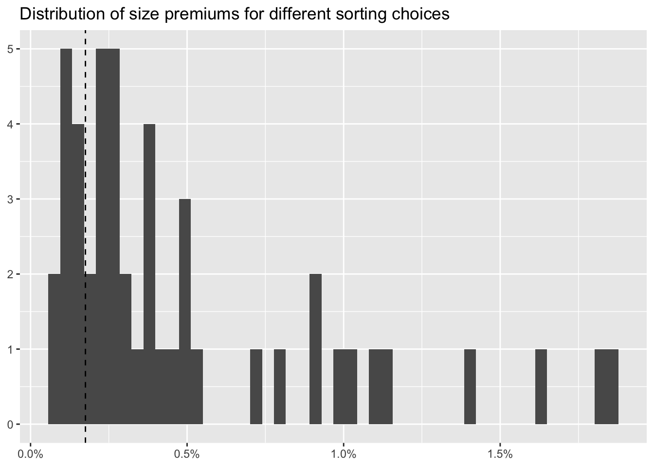
Finally, we close the database.
dbDisconnect(tidy_finance, shutdown = TRUE)