Solutions for Panel data

Updated Python Polars solutions

These solutions accompany the Panel data chapter of Empirical Research in Accounting: Tools and Methods. This notes edition updates the solutions discussed in the original 2026-05-20 post with subsequent corrections and clarifications; it is not a facsimile of the original LinkedIn attachment. The calculations were freshly executed on 26 October 2026.

The calculations use a local Parquet repository, with DATA_DIR pointing to that repository. See the book’s data setup instructions and the accompanying Python requirements. The QMD uses the existing era_pl_sols Jupyter kernel, whose environment supplies those packages; its code does not import either solutions repository. Changes in the input data or software can change estimates and timings.

1 Exercises

1. Generate a random sample of test scores using get_test_scores() with some value of effect_size and some value of seed. Assign this to the variable df_1. Estimate the model "score ~ I(treat * post) | grade + id" using pf.feols() with data=df_1 and vcov="iid" and store the result in fm. Compare the output of fm.tidy() with that from fit_test_score_panel(df_1, vcov="iid"). What do you observe?

   Estimate the model "score ~ I(treat * post) | grade + id" using pf.feols() with data=df_1 and vcov={"CRV1": "grade + id"} and store the result in fm2. Compare the output of fm2.tidy() with that from fit_test_score_panel(df_1, vcov={"CRV1": "grade + id"}). What do you observe?

df_1 = get_test_scores(effect_size=0.1, seed=100)

fm = pf.feols(
    "score ~ I(treat * post) | grade + id",
    data=df_1,
    vcov="iid",
)

fm2 = pf.feols(
    "score ~ I(treat * post) | grade + id",
    data=df_1,
    vcov={"CRV1": "grade + id"},
)

fit_test_score_panel(df_1, vcov="iid")

shape: (1, 4)

estimate	se	t	p_value
f64	f64	f64	f64
1.000819	0.31368	3.190576	0.001435

fit_test_score_panel(df_1, vcov={"CRV1": "grade + id"})

shape: (1, 4)

estimate	se	t	p_value
f64	f64	f64	f64
1.000819	0.930173	1.075949	0.360774

The outputs match the corresponding rows from fm.tidy() and fm2.tidy() for the treatment-effect coefficient. The helper returns just the quantities needed for the simulation analysis: the estimate, standard error, \(t\)-statistic, and \(p\)-value.

2. Given the above, why do you think we included fit_test_score_panel() rather than using pf.feols()? Develop and run a test of your hypothesis for why we did so.

The likely reason is speed. The chapter runs the same two-way fixed-effects regression many times in simulation, and fit_test_score_panel() is specialized to this exact setting. The following code compares the two approaches over a modest number of replications.

import time

num_runs = 50
sim_dfs = [
    get_test_scores(effect_size=0, seed=i)
    for i in range(num_runs)
]

start = time.perf_counter()
_ = [
    pf.feols(
        "score ~ I(treat * post) | grade + id",
        data=df,
        vcov="iid",
    ).coef()["I(treat * post)"]
    for df in sim_dfs
]
pyfixest_time = time.perf_counter() - start

start = time.perf_counter()
_ = [
    fit_test_score_panel(df, vcov="iid").item(0, "estimate")
    for df in sim_dfs
]
helper_time = time.perf_counter() - start

pl.DataFrame({
    "method": ["pyfixest", "fit_test_score_panel"],
    "seconds": [pyfixest_time, helper_time],
    "runs": [num_runs, num_runs],
}).with_columns(
    seconds_per_run=pl.col("seconds") / pl.col("runs")
).with_columns(
    pl.col("seconds", "seconds_per_run").round(4)
).style

Table 1: Timing comparison for simulated panel regressions

method	seconds	runs	seconds_per_run
pyfixest	0.264	50	0.0053
fit_test_score_panel	0.0085	50	0.0002

The timing table measures the relative speed of the helper and the general estimator in this run. The exact times depend on the computer, software versions and workload. That speed matters because the chapter uses 1,000 replications in several settings.

2 Discussion questions

1. The proprietary cost hypothesis tested by Li et al. (2018) posits that increased cost of disclosure will lead to reduced supply of disclosure. What rival theories exist that would make alternative predictions? Are there other elements of disclosure theory that might be tested? Why do you think Li et al. (2018) focused on this specific element of the proprietary cost hypothesis?

There are no clear rival theories other than “no effect”. Of course, “no effect” is unlikely to be found in a published paper for reasons discussed in Chapter 19. There are other elements of the theory that might be examined, such as the firms with good news (observed in later realizations) being the ones who disclose and the market reacting favourably to disclosure. At times it seems the least interesting aspect of “proprietary cost hypothesis” gets studied again and again in “increasingly clever” ways.

2. In the analysis above, we do not include the control variables considered by Li et al. (2018). For example, Li et al. (2018) “include R&D expenditures to sales, advertisement [sic] expenditure to sales, and intangible assets scaled by total assets to control for a firm’s proprietary costs of disclosure.” Using the approach outlined in Chapter 4, in what circumstances would it be necessary to control for “a firm’s proprietary costs of disclosure” in this way? Do these circumstances seem applicable in this setting, where the treatment is a (presumably exogenous) shock to disclosure costs and the outcome is disclosure choices?

The first question is whether a proposed control is a pre-treatment common cause, a precision variable, or a variable affected by IDD. Controlling for proprietary costs changed by IDD could block the proposed mechanism. A better interpretation is simply that the wording used by Li et al. (2018) is poor. Instead, Li et al. (2018) are in effect using IDD adoption as an exogenous shock to the treatment. This is like using IDD adoption as an instrument, but focused on intent-to-treat analyses.¹

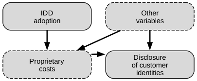
Intent-to-treat analyses are common when researchers have an instrument, but do not observe the treatment of interest directly.² In this setting, the treatment of interest is “proprietary costs of disclosure” and a maintained assumption is that IDD adoption is random, has a direct causal effect on proprietary costs of disclosure, and does not affect the outcome (in this setting, voluntary disclosure of customer identities) except through its effect on the treatment. This can be represented on a causal diagram as in Figure 1.

In conventional IV analyses, it is considered a standard step to evaluate the relationship between the instrument (\(Z\)) and the treatment (\(X\)) statistically.³ But this is not possible when the treatment is not observed. As such, in addition to assumptions about the causal relationship between \(Z\) and \(X\), the magnitude of the proprietary-cost change is unobserved. A reduced-form effect of IDD exposure does not require dividing by a measured first stage, but it does not identify the effect per unit of proprietary costs. So we need to assume that IDD adoption has a causal effect on proprietary costs of disclosure and the empirical tests are joint tests of that assumption and the hypothesis that increased costs of disclosure lead to reduced supply of disclosure.⁴

Figure 1: Causal diagram for Li et al. (2018)

The variables that need to be controlled for are any determinants of “a firm’s proprietary costs of disclosure” that also affect the instrument. If IDD exposure were randomly assigned, baseline controls could improve precision. If it is only as-if random conditional on measured factors, those factors matter for identification; time-varying confounders and conditional parallel trends remain relevant. Post-treatment measures of proprietary costs should not be added mechanically. But Li et al. (2018) no doubt understood that in accounting research it’s important to “control for stuff”.

3. What differs between the regressions reported in columns (1) and (3), and (2) and (4) of Table 2, respectively? Does this tell you anything about what drives the regression results in this setting? What happens if you omit the year fixed effects from both sets of regressions? What does this tell you about the role of the “non-switchers” (i.e., firms not in the switchers data frame) in the regression?

In the regression output below, warnings from pyfixest about singleton fixed effects and collinear event-time indicators are suppressed. These warnings reflect observations or indicators that the fixed-effects estimator drops automatically; they do not affect the interpretation of the reported coefficients.

Table 2: Effect of IDD adoption

	ln_ratio	ln_ratio_sale	ln_ratio	ln_ratio_sale
	(1)	(2)	(3)	(4)
coef
post	0.016** (0.008)	0.024*** (0.008)	0.014 (0.009)	0.019** (0.01)
fe
gvkey	x	x	x	x
year	x	x	x	x
stats
Sample	All	All	Switchers	Switchers
Observations	28,230	23,923	3,611	3,154
R2	0.665	0.703	0.623	0.66
Significance levels: * p < 0.1, ** p < 0.05, *** p < 0.01. Format of coefficient cell: Coefficient (Std. Error)

What differs between the regressions reported in columns (1) and (3), and (2) and (4) of Table 2, respectively?

The samples are different. Columns (1) and (2) include all firms, while columns (3) and (4) only include the “switchers” (defined above as firms whose treatment status changed during the sample period).

What happens if you omit the year fixed effects from both sets of regressions?

It is easy to tweak the code to omit year fixed effects:

fms_no_year = [
    pf.feols("ln_ratio ~ post | gvkey", data=reg_data, vcov="iid"),
    pf.feols("ln_ratio_sale ~ post | gvkey", data=reg_data, vcov="iid"),
    pf.feols("ln_ratio ~ post | gvkey", data=reg_data_switchers, vcov="iid"),
    pf.feols("ln_ratio_sale ~ post | gvkey", data=reg_data_switchers, vcov="iid"),
]

Results are reported in Table 3. Without year fixed effects, the treatment coefficients agree between the full and switcher samples. The observation counts and standard errors can differ, so the complete regression results are not identical.

Table 3: Effect of IDD adoption: No year fixed effects

	ln_ratio	ln_ratio_sale	ln_ratio	ln_ratio_sale
	(1)	(2)	(3)	(4)
coef
post	0.026*** (0.008)	0.025*** (0.008)	0.026*** (0.008)	0.025*** (0.008)
fe
gvkey	x	x	x	x
stats
Sample	All	All	Switchers	Switchers
Observations	28,230	23,923	3,611	3,154
R2	0.664	0.702	0.619	0.657
Significance levels: * p < 0.1, ** p < 0.05, *** p < 0.01. Format of coefficient cell: Coefficient (Std. Error)

What does this tell you about what drives the regression results in this setting?

Regression results are driven by the switchers.

What does this tell you about the role of the “non-switchers” (i.e., firms not in the switchers data frame) in the regression?

This tells us that the only impact of the “non-switchers” on the full regression results is via their effect on the estimated year fixed effects. These firms do not directly affect the estimates of the treatment effect or of other firms’ fixed effects, which are driven by the switchers and the individual firms, respectively.

4. Would you expect the inclusion of controls (see the question above) to have a significant impact on the regression results? Why or why not?

I would not expect the controls to have a big impact for a number of reasons. First, many controls would be fairly persistent over time and, with firm fixed effects included, only within-firm variation in controls that is correlated with the treatment indicator (i.e., POST for treatment firms) will affect the estimated effects.

With firm fixed effects, only within-firm variation in controls can change the treatment estimate. Persistence makes a small effect plausible when the remaining variation is weakly related to treatment, but it is not a guarantee. A time-varying omitted confounder can still matter. State effects provide a useful sensitivity check because firms sometimes change headquarters state; the paper includes state effects in its specification. When making that comparison, hold the estimation sample and covariance convention fixed first, so that changes in the coefficient are not confused with changes in the sample or standard errors.

5. What differs between the regressions reported in columns (1) and (3), and (2) and (4) of Table 4, respectively? What happens if you omit the year fixed effects from both sets of regressions? What does this tell you about what drives the regression results in this setting?

Table 4: Effect of IDD adoption by year

	ln_ratio	ln_ratio_sale	ln_ratio	ln_ratio_sale
	(1)	(2)	(3)	(4)
coef
t = -5	-0.004 (0.019)	0.001 (0.021)	-0.017 (0.027)	-0.009 (0.029)
t = -4	-0.018 (0.022)	-0.031 (0.023)	-0.026 (0.025)	-0.038 (0.026)
t = -3	-0.03 (0.02)	-0.029 (0.02)	-0.031 (0.021)	-0.031 (0.022)
t = -2	-0.009 (0.018)	-0.003 (0.018)	-0.014 (0.019)	-0.01 (0.019)
t = 0	-0.000882 (0.015)	0.016 (0.015)	0.007 (0.016)	0.02 (0.017)
t = 1	0.009 (0.016)	0.025 (0.017)	0.021 (0.018)	0.031 (0.02)
t = 2	-0.008 (0.017)	0.01 (0.018)	0.009 (0.021)	0.017 (0.023)
t = 3	0.023 (0.019)	0.021 (0.02)	0.038 (0.025)	0.026 (0.027)
t = 4	0.028 (0.019)	0.039* (0.021)	0.041 (0.027)	0.042 (0.03)
t = 5	0.043*** (0.015)	0.048*** (0.016)	0.046 (0.032)	0.039 (0.036)
fe
gvkey	x	x	x	x
year	x	x	x	x
stats
Sample	All	All	Switchers	Switchers
Observations	28,230	23,923	3,104	2,732
R2	0.666	0.703	0.624	0.667
Significance levels: * p < 0.1, ** p < 0.05, *** p < 0.01. Format of coefficient cell: Coefficient (Std. Error)

What happens if you omit the year fixed effects from both sets of regressions?

Here is the code to estimate regressions without year fixed effects.

fms_year_no_year = [
    pf.feols("ln_ratio ~ C(t, Treatment(reference=-1)) | gvkey",
             data=reg_data_t, vcov="iid"),
    pf.feols("ln_ratio_sale ~ C(t, Treatment(reference=-1)) | gvkey",
             data=reg_data_t, vcov="iid"),
    pf.feols("ln_ratio ~ C(t, Treatment(reference=-1)) | gvkey",
             data=reg_data_t.filter(pl.col("t").is_finite()), vcov="iid"),
    pf.feols("ln_ratio_sale ~ C(t, Treatment(reference=-1)) | gvkey",
             data=reg_data_t.filter(pl.col("t").is_finite()), vcov="iid"),
]

As can be seen in the results reported in Table 5, only the firms that are treated for part of the sample drive the regression results absent year fixed effects. We have identical coefficients in columns (1) and (3), and in columns (2) and (4).

Table 5: Effect of IDD adoption by year: No year fixed effects

	ln_ratio	ln_ratio_sale	ln_ratio	ln_ratio_sale
	(1)	(2)	(3)	(4)
coef
t = -5	-0.012 (0.019)	0.003 (0.02)	-0.012 (0.019)	0.003 (0.021)
t = -4	-0.03 (0.022)	-0.035 (0.023)	-0.03 (0.022)	-0.035 (0.023)
t = -3	-0.04** (0.02)	-0.033 (0.02)	-0.04* (0.02)	-0.033 (0.021)
t = -2	-0.013 (0.018)	-0.005 (0.018)	-0.013 (0.018)	-0.005 (0.018)
t = 0	0.005 (0.015)	0.019 (0.015)	0.005 (0.015)	0.019 (0.015)
t = 1	0.018 (0.016)	0.028* (0.017)	0.018 (0.016)	0.028* (0.017)
t = 2	0.004 (0.017)	0.011 (0.018)	0.004 (0.017)	0.011 (0.018)
t = 3	0.033* (0.018)	0.02 (0.02)	0.033* (0.019)	0.02 (0.02)
t = 4	0.035* (0.019)	0.032 (0.021)	0.035* (0.02)	0.032 (0.021)
t = 5	0.045*** (0.014)	0.032** (0.015)	0.045*** (0.014)	0.032** (0.015)
fe
gvkey	x	x	x	x
stats
Sample	All	All	Switchers	Switchers
Observations	28,230	23,923	3,104	2,732
R2	0.664	0.702	0.62	0.665
Significance levels: * p < 0.1, ** p < 0.05, *** p < 0.01. Format of coefficient cell: Coefficient (Std. Error)

6. What patterns do you observe in the coefficients reported in Table 4? Do these conform to what you would expect from Li et al. (2018)? (It may be easiest to focus on these in groups, e.g., those in \(t-5\) to \(t-2\), those in \(t + 0\) to \(t+3\) and those for \(t+4\) and \(t+5\).)

In Table 4, most pre-adoption coefficients are negative, while the clearest positive signal in the full sample is in the pooled \(t+5\)-and-later bin. The weighted measure is only marginally significant at \(t+4\); results for firms observed to switch differ. The estimates and their uncertainty should be read together, rather than treating a sign as evidence of a nonzero effect.

These do not conform with what I’d expect from reading Li et al. (2018). First, the negative coefficients in years \(t-5\) through \(t-2\) are problematic, but their signs alone do not establish anticipation or rejection of parallel trends. Their uncertainty and a joint test of the leads should also be examined. Second, the clearest positive signals appear relatively late in this expanded specification. Li et al. (2018) discuss effects within one or two years [pp. 269 and 288], so it is inaccurate to say that the paper does not discuss delay. Table 3 pools observations from \(t+2\) onward and cannot identify onset within that pooled period. Online appendix Table OA2 uses a \([-2,+2]\) window and reports significant coefficients at exactly \(t+2\), with a matched sample and a different reference year. Our later pattern is a discrepancy to investigate, rather than a direct contradiction of estimates from that different design.

The number and composition of firms vary by event year. The later coefficients rely on fewer firms, and a pooled tail can contain several observations from each firm. Report firm counts as well as row counts before judging how much independent support a late-period estimate has.

7. How do the variables in Table 4 differ from those used in Table 3 of Li et al. (2018)? Modify the code above (e.g., format_event_time()) to produce analysis closer to that reported in Table 3 of Li et al. (2018).

Li et al. (2018) treat years before \(t-2\) the same as years without treatment and collapse years after \(t+2\) into year \(t+2\). We can replace the regression above by using a modified format_event_time() as follows. This function pools the years before \(t - 2\) with the control firms by setting their level at \(-\infty\) and caps the upper event-time indicator at \(t + 2\).

The other thing that Li et al. (2018) do is report coefficients relative to non-treatment firms and firm-years strictly before \(t-2\) (some reference group needs to be chosen), which we implement by pooling pre-\(t-2\) treated firm-years with the control group.

def format_event_time_llz(value):
    if value is None or value < -2:
        return -np.inf
    value = int(value)
    return float(min(2, value))

reg_data_t_llz = (
    reg_data
    .join(switch_years, on="gvkey", how="left")
    .with_columns(
        (pl.col("year") - pl.col("adoption_year"))
        .map_elements(
            format_event_time_llz,
            return_dtype=pl.Float64,
            skip_nulls=False,
        )
        .alias("t_llz"),
    )
)

fms_llz = [
    pf.feols("ln_ratio ~ C(t_llz, Treatment(reference=-np.inf)) "
             "| gvkey + year",
             data=reg_data_t_llz, vcov="iid"),
    pf.feols("ln_ratio_sale ~ C(t_llz, Treatment(reference=-np.inf)) "
             "| gvkey + year",
             data=reg_data_t_llz, vcov="iid"),
]

Table 6: Effect of IDD adoption by year

	ln_ratio	ln_ratio_sale
	(1)	(2)
coef
t = -2	0.008 (0.017)	0.015 (0.017)
t = -1	0.016 (0.015)	0.018 (0.016)
t = 0	0.015 (0.014)	0.034** (0.015)
t = 1	0.024 (0.016)	0.043** (0.017)
t = 2	0.042*** (0.013)	0.05*** (0.014)
fe
gvkey	x	x
year	x	x
stats
Observations	28,230	23,923
R2	0.665	0.703
Significance levels: * p < 0.1, ** p < 0.05, *** p < 0.01. Format of coefficient cell: Coefficient (Std. Error)

The positive pooled coefficients in Table 6 have the same broad direction as Table 3 of Li et al. (2018). These regressions retain IID standard errors and change the event coding only, so their significance cannot be described as stronger evidence than the paper’s differently clustered specification. The net effect of the reporting choices made here appears to be to collapse the effects of \(t+3\), \(t+4\), and \(t+5\) into \(t+2\) and to suppress the reporting of any of the awkward negative coefficients in years \(t-5\) through \(t-3\).

This changes the event coding, but it does not reproduce the paper’s full specification. We retain the book’s controls, missing-value handling and first observed pre-to-post transition as the event year. That transition can reflect a headquarters change or an observation gap, whereas the paper’s indicators refer to state adoption years. The authors’ supplied code replaces missing weighted ratios with one; our code retains them as missing. State effects, state-clustered inference and sample restrictions are further distinct choices.

A significant coefficient on the pooled \(t+2\)-and-later category does not establish that an effect begins at exactly \(t+2\). It averages the later years too, while pooling early years into the reference removes their separate estimates from view. Assess the displayed comparison with these differences in mind.

8. The format_event_time() function collapses years after \(t + 5\) and before \(t - 5\) into years \(t + 5\) and \(t - 5\), respectively. When would this approach make sense? What would be one alternative approach to handling these years? Does your suggested approach make a difference in this setting?

Binning can make sense when very early and late event years contain few observations, so separate estimates would be unstable and hard to interpret. Pooling gives more precise tail estimates, but imposes a common effect on all years in each tail. It is most defensible when that approximation is plausible and the research question concerns the years near adoption. It can conceal changes or reversals in distant years, so the bin definitions and sensitivity to them should be reported.

One alternative approach would be not to collapse them at all and report them separately. Here we use the format_event_time_all() function defined above, which implements this idea.

def format_event_time_all(value):
    if value is None:
        return -np.inf
    return float(int(value))

reg_data_t_all = (
    reg_data
    .join(switch_years, on="gvkey", how="left")
    .with_columns(
        (pl.col("year") - pl.col("adoption_year"))
        .map_elements(
            format_event_time_all,
            return_dtype=pl.Float64,
            skip_nulls=False,
        )
        .alias("t_all"),
    )
)

fms_all_years = [
    pf.feols("ln_ratio ~ C(t_all, Treatment(reference=-1)) "
             "| gvkey + year",
             data=reg_data_t_all, vcov="iid"),
    pf.feols("ln_ratio_sale ~ C(t_all, Treatment(reference=-1)) "
             "| gvkey + year",
             data=reg_data_t_all, vcov="iid"),
    pf.feols("ln_ratio ~ C(t_all, Treatment(reference=-1)) "
             "| gvkey + year",
             data=reg_data_t_all.filter(pl.col("t_all").is_finite()), vcov="iid"),
    pf.feols("ln_ratio_sale ~ C(t_all, Treatment(reference=-1)) "
             "| gvkey + year",
             data=reg_data_t_all.filter(pl.col("t_all").is_finite()), vcov="iid"),
]

Table 7: Effect of IDD adoption by year (all years)

	ln_ratio	ln_ratio_sale	ln_ratio	ln_ratio_sale
	(1)	(2)	(3)	(4)
coef
t = -15	0.317**	0.23	0.242	0.177
t = -14	0.261	0.088	0.239	0.073
t = -13	-0.026		-0.08
t = -12	-0.471**		-0.529
t = -11	-0.227***	-0.21***	-0.255	-0.24
t = -10	-0.128**	-0.153**	-0.147	-0.165
t = -9	-0.072	-0.067	-0.088	-0.083
t = -8	-0.009	0.064	-0.022	0.051
t = -7	0.117***	0.16***	0.096	0.139
t = -6	0.034	0.037	0.014	0.017
t = -5	-0.025	-0.036	-0.045	-0.057
t = -4	-0.018	-0.032	-0.031	-0.046
t = -3	-0.03	-0.03	-0.034	-0.036
t = -2	-0.008	-0.003	-0.017	-0.013
t = 0	-0.001	0.016	0.007	0.021
t = 1	0.008	0.025	0.023	0.036
t = 2	-0.008	0.011	0.013	0.025
t = 3	0.022	0.022	0.043	0.035
t = 4	0.027	0.039*	0.047	0.053
t = 5	0.04*	0.037*	0.063	0.054
t = 6	0.029	0.041*	0.047	0.052
t = 7	0.05**	0.053**	0.061	0.062
t = 8	0.054**	0.057**	0.068	0.068
t = 9	0.042*	0.028	0.047	0.029
t = 10	0.039	0.04	0.042	0.041
t = 11	0.077**	0.099***	0.082	0.095
t = 12	0.072**	0.097**	0.071	0.09
t = 13	0.05	0.097*	0.055	0.093
t = 14	-0.033	-0.04	-0.033	-0.05
t = 15	-0.011	0.058	-0.016	0.037
fe
gvkey	x	x	x	x
year	x	x	x	x
stats
Sample	All	All	Switchers	Switchers
Observations	28,230	23,923	3,104	2,732
R2	0.666	0.704	0.63	0.673
Significance levels: * p < 0.1, ** p < 0.05, *** p < 0.01. Format of coefficient cell: Coefficient

But, as can be seen in the results reported in Table 7, this level of transparency makes the results seem even more difficult to explain.⁵

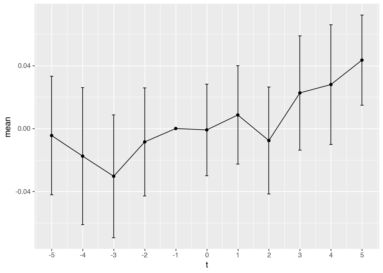
9. How helpful do you find Figure 2 (plot of the coefficients by year)?

plot_coefs(fms_year[0])

Figure 2: Plot of coefficients by year

It’s somewhat helpful, but it’s really just the “by year” regression results in graphical form. I’m not inclined to believe any of the results in Li et al. (2018) given where these results are coming from … and I don’t need the plot to tell me that. I think that if the results were (in my view, counterfactually) real, a plot like this might be a useful way to communicate that.

10. Describe the data set created from the following code. What proportion of the firms in the data set have same_state equal to true? For the purposes of empirical analysis, do the firms with same_state equal to false enhance, or detract from, our ability to draw causal inferences about the effect of adoption of IDD?

switch_years_state = (
    reg_data_switchers
    .sort(["gvkey", "datadate"])
    .with_columns(
        pl.col("state", "period_type").shift(1).over("gvkey")
        .name.prefix("lag_")
    )
    .with_columns(
        same_state=pl.col("state") == pl.col("lag_state"),
        adoption_year=
            (pl.col("period_type") == "Post-adoption") &
            (pl.col("lag_period_type") == "Pre-adoption"),
    )
    .filter(pl.col("adoption_year"))
)

switch_years_state.group_by("same_state").agg(n=pl.len())

shape: (2, 2)

same_state	n
bool	u32
true	251
false	134

A firm can contribute more than one observed pre-to-post transition, so the proportion of records is not necessarily the proportion of firms. The following calculation distinguishes all transition records, firms with at least one unchanged-state transition, and each firm’s first transition.

firm_transitions = switch_years_state.group_by("gvkey").agg(
    any_same_state=pl.col("same_state").fill_null(False).any()
)
first_transitions = (
    switch_years_state.sort(["gvkey", "datadate"])
    .unique("gvkey", keep="first", maintain_order=True)
)
state_transition_summary = pl.DataFrame({
    "Unit": ["Transition records", "Firms: at least one", "Firms: first transition"],
    "Unchanged state": [
        switch_years_state["same_state"].sum(),
        firm_transitions["any_same_state"].sum(),
        first_transitions["same_state"].sum(),
    ],
    "Total": [
        switch_years_state.height,
        firm_transitions.height,
        first_transitions.height,
    ],
}).with_columns(Share=pl.col("Unchanged state") / pl.col("Total"))
state_transition_summary.style.fmt_integer(
    columns=["Unchanged state", "Total"]
).fmt_percent(columns="Share", decimals=1)

Unit	Unchanged state	Total	Share
Transition records	251	385	65.2%
Firms: at least one	251	382	65.7%
Firms: first transition	250	382	65.4%

same_state is true when the headquarters state is unchanged from the preceding observed record and false when the transition coincides with a recorded state change. The first-transition calculation follows the book’s event-year convention; the “at least one” calculation answers a different firm-level question.

The changed-state cases weaken the claim that every exposure change comes from an exogenous court ruling in a firm’s existing state. They can reflect endogenous relocation, but location-record changes, mergers and other events may also explain them; these records alone do not establish intentional relocation. They may add statistical variation while making causal interpretation harder. Useful sensitivity checks restrict transitions to unchanged-state firms or fix headquarters location before the ruling, while acknowledging the resulting selection and measurement issues.

11. What issues might be implied by the following data? How might you address these?

(
    reg_data_t
    .group_by("t")
    .agg(n=pl.len().alias("n"))
    .sort("t")
    .style
    .fmt_integer()
)

t	n
−inf	25,603
−5	232
−4	116
−3	153
−2	218
−1	321
0	384
1	305
2	233
3	192
4	168
5	782

One issue is that the sample is changing from one event-period to the next. Requiring observation at \(t+4\) does not ensure a balanced panel at all earlier event times, and it excludes the never-switching comparison pool. A balanced-window sensitivity analysis must explicitly require each desired event year and separately retain an appropriate control pool. One idea would be to require that a firm be in the sample in \(t + 4\) (the full and switcher samples play different roles once year effects are included) and to drop all periods after \(t + 4\) and run the by-year regressions for this sample.

reg_data_t2 = (
    reg_data_t
    .filter(pl.col("t") == 4)
    .select("gvkey")
    .unique()
    .join(reg_data_t, on="gvkey", how="inner")
    .filter(pl.col("t") < 5)
)

fms_constant = [
    pf.feols("ln_ratio ~ C(t, Treatment(reference=-1)) "
             "| gvkey + year",
             data=reg_data_t2, vcov="iid"),
    pf.feols("ln_ratio_sale ~ C(t, Treatment(reference=-1)) "
             "| gvkey + year",
             data=reg_data_t2, vcov="iid"),
]

Using the code above to create this sample, regression results are reported in Table 8. Perhaps unsurprisingly there are no consistent results here.

Table 8: Effect of IDD adoption by year: Firms observed at \(t+4\)

	ln_ratio	ln_ratio_sale
	(1)	(2)
coef
t = -5	-0.011 (0.081)	-0.147 (0.095)
t = -4	-0.026 (0.055)	-0.105 (0.064)
t = -3	-0.036 (0.041)	-0.084* (0.047)
t = -2	-0.004 (0.03)	-0.038 (0.033)
t = 0	0.015 (0.027)	0.055* (0.03)
t = 1	0.028 (0.037)	0.087** (0.043)
t = 2	-0.014 (0.049)	0.064 (0.059)
t = 3	-0.023 (0.062)	0.076 (0.075)
t = 4	-0.018 (0.075)	0.112 (0.092)
fe
gvkey	x	x
year	x	x
stats
Observations	1,237	1,126
R2	0.667	0.693
Significance levels: * p < 0.1, ** p < 0.05, *** p < 0.01. Format of coefficient cell: Coefficient (Std. Error)

The \(t+4\) restriction also selects on later survival and data availability. A fully balanced event window would require exactly one complete observation in every chosen event year for both outcomes, then retain an appropriate comparison pool. Report the number of qualifying treated firms and support by adoption cohort: balancing can sharply reduce the available sample. Neither balancing nor the selected \(t+4\) sample resolves heterogeneous treatment effects in a staggered-adoption design. The changing sample, a sample selected at \(t+4\), and a balanced-window sample answer different questions.

3 References

Bloomfield, M.J., 2021. The asymmetric effect of reporting flexibility on priced risk. Journal of Accounting Research 59, 867–910. https://doi.org/10.1111/1475-679X.12346

Hoekstra, M., 2009. The effect of attending the flagship state university on earnings: A discontinuity-based approach. The Review of Economics and Statistics 91, 717–724. https://doi.org/10.1162/rest.91.4.717

Li, Y., Lin, Y., Zhang, L., 2018. Trade secrets law and corporate disclosure: Causal evidence on the proprietary cost hypothesis. Journal of Accounting Research 56, 265–308. https://doi.org/10.1111/1475-679X.12187

Footnotes

1. Recall from Table 1 of Hoekstra (2009) that an intent-to-treat analysis regresses the outcome directly on the instrument.

2. Bloomfield (2021) focuses on intent-to-treat analyses, even though the treatment is observed.

3. As always, remember that the critical assumption is causal not statistical, but statistical analysis is necessary to check for problems in the finite-sample behaviour of IV analyses.

4. My own view is that it is quite obvious that increased costs of disclosure lead to reduced supply of disclosure and that the paper is really a test of the effect of IDD adoption on proprietary costs of disclosure. For reasons that will become evident by the end of this document, I think the evidence from the setting in Li et al. (2018) is very far from persuasive.

5. Note that the results obtained from running the equivalent code in R differ for columns (3) and (4) because the R code omits the \(t + 15\) indicator due to collinearity and the Python code makes a different choice. This has no impact on the substance of the results.