A quick look at City of Melbourne bike data

Author

Ian D. Gow

Published

19 September 2024

In writing this note, I use the packages listed below.¹ This note was written using Quarto and compiled with RStudio, an integrated development environment (IDE) for working with R. The source code for this note is available here and the latest version of this PDF is here.²

library(tidyverse)
library(duckdb)
library(tinytable)

The following code downloads the data and unzips the single file therein. It is cached (cache: true in chunk options) to save time with repeated runs of the code.

t <- tempfile(fileext = ".zip")
url <- str_c("https://opendatasoft-s3.s3.amazonaws.com/",
             "downloads/archive/74id-aqj9.zip")
download.file(url, t)
unzip(t)

I create a database connection and load the icu extension, which contains time-zone information.³

db <- dbConnect(duckdb::duckdb(), timezone_out = "Australia/Melbourne")
dbExecute(db, "INSTALL icu")
dbExecute(db, "LOAD icu")

The following SQL creates bikes_raw, which is fairly unprocessed data. Only RUNDATE is given a type, and this is TIMESTAMP because there is no time zone information in the data.

CREATE OR REPLACE TABLE bikes_raw AS
  SELECT *
  FROM read_csv('74id-aqj9.csv',
                timestampformat='%Y%m%d%H%M%S',
                types={'RUNDATE': 'TIMESTAMP'});

The following SQL produces some information on the contents of bikes_raw that is shown in Table 1.

SELECT column_name, column_type, max, null_percentage
FROM (SUMMARIZE bikes_raw);

Table 1: Information on unprocessed data (bikes_raw)

column_name	column_type	max	null_percentage
ID	BIGINT	57	0.00
NAME	VARCHAR	Yorkshire Brewery - Wellington St - Collingwood	0.00
TERMINALNAME	BIGINT	60052	0.00
NBBIKES	BIGINT	39	0.00
NBEMPTYDOCKS	BIGINT	39	0.00
RUNDATE	TIMESTAMP	2018-09-04 10:00:10	0.00
INSTALLED	BOOLEAN	true	0.00
TEMPORARY	BOOLEAN	false	0.00
LOCKED	BOOLEAN	true	0.00
LASTCOMMWITHSERVER	BIGINT	1507119446229	0.00
LATESTUPDATETIME	BIGINT	1507119264599	0.02
REMOVALDATE	VARCHAR	NA	100.00
INSTALLDATE	BIGINT	1450061460000	22.01
LAT	DOUBLE	-37.79625	0.00
LONG	DOUBLE	144.988507	0.00
LOCATION	VARCHAR	(-37.867068, 144.976428)	0.00

The following function is created in R, but generates SQL. The documentation for make_timestamptz() says that it returns “the TIMESTAMP WITH TIME ZONE for the given µs since the epoch.” But it seems the data we have are in milliseconds, not microseconds, so we need to multiply by 1000.

epoch_to_ts <- function(x) {
  x <- rlang::as_name(rlang::enquo(x))
  dplyr::sql(stringr::str_c("make_timestamptz(", x, " * 1000)"))
}

The following code converts rundate to TIMESTAMPTZ assuming the original data are Melbourne times. It also converts lastcommwithserver, latestupdatetime, and installdate to TIMESTAMPTZ. Note that attention needs to be paid to time zones, because the epoch is defined as “the number of seconds since 1970-01-01 00:00:00 UTC”, which would be a different point in time from 1970-01-01 00:00:00 in Melbourne time.

bikes <-
  tbl(db, "bikes_raw") |>
  rename_with(str_to_lower) |>
  select(-installed, -temporary, -removaldate) |>
  mutate(rundate = timezone("Australia/Melbourne", rundate),
         lastcommwithserver = !!epoch_to_ts(lastcommwithserver),
         latestupdatetime = !!epoch_to_ts(latestupdatetime),
         installdate = !!epoch_to_ts(installdate)) |>
  compute(name = "bikes", overwrite = TRUE)

The following SQL produces some information on the contents of bikes that is shown in Table 2.

SELECT column_name, column_type, max, null_percentage
FROM (SUMMARIZE bikes);

Table 2: Information on processed data (bikes)

column_name	column_type	max	null_percentage
id	BIGINT	57	0.00
name	VARCHAR	Yorkshire Brewery - Wellington St - Collingwood	0.00
terminalname	BIGINT	60052	0.00
nbbikes	BIGINT	39	0.00
nbemptydocks	BIGINT	39	0.00
rundate	TIMESTAMP WITH TIME ZONE	2018-09-03 20:00:10-04	0.00
locked	BOOLEAN	true	0.00
lastcommwithserver	TIMESTAMP WITH TIME ZONE	2017-10-04 08:17:26.229-04	0.00
latestupdatetime	TIMESTAMP WITH TIME ZONE	2017-10-04 08:14:24.599-04	0.02
installdate	TIMESTAMP WITH TIME ZONE	2015-12-13 21:51:00-05	22.01
lat	DOUBLE	-37.79625	0.00
long	DOUBLE	144.988507	0.00
location	VARCHAR	(-37.867068, 144.976428)	0.00

bikes |> 
  select(lastcommwithserver, latestupdatetime, rundate, installdate) |>
  collect(n = 10)

Table 3: Sample of date-time variables

lastcommwithserver	latestupdatetime	rundate	installdate
2017-04-22 13:42:46.01	2017-04-22 13:42:45.029	2017-04-22 13:45:06	2011-08-19 13:30:00
2017-04-22 13:43:51.727	2017-04-22 13:36:17.573	2017-04-22 13:45:06	NA
2017-04-22 13:33:35.231	2017-04-22 13:33:33.615	2017-04-22 13:45:06	NA
2017-04-22 13:36:58.661	2017-04-22 12:51:55.84	2017-04-22 13:45:06	NA
2017-04-22 13:35:03.674	2017-04-21 19:56:38.168	2017-04-22 13:45:06	NA
2017-04-22 13:32:35.565	2017-04-22 13:18:29.294	2017-04-22 13:45:06	2012-12-27 08:00:00
2017-04-22 13:41:32.347	2017-04-22 11:55:01.271	2017-04-22 13:45:06	NA
2017-04-22 13:34:42.173	2017-04-22 13:34:40.671	2017-04-22 13:45:06	NA
2017-04-22 13:36:33.207	2017-04-22 11:49:37.265	2017-04-22 13:45:06	NA
2017-04-22 13:37:50.326	2017-04-22 13:37:48.824	2017-04-22 13:45:06	2010-06-22 12:53:00

In making Figure 1, I convert the date component of runtime to the same date (2017-01-01). This facilitates plotting in R, as R has no native “time” type and thus things are easier using date-times. Unfortunately, it seems that all the timestamps in bikes are boring back-end times produced by systems, so there is nothing special about the distribution of these times. More interest plots might come from looking at when bikes are checked out and in (only net checkouts seem to be available) assuming that the data are sufficiently frequent.

bikes |>
  mutate(runtime = make_timestamptz(2017L, 1L, 1L, 
                                    hour(rundate), minute(rundate), 
                                    second(rundate))) |>
  ggplot(aes(runtime)) +
  geom_histogram(binwidth = 60 * 60) +
  scale_x_datetime(date_breaks = "1 hour", date_labels = "%H")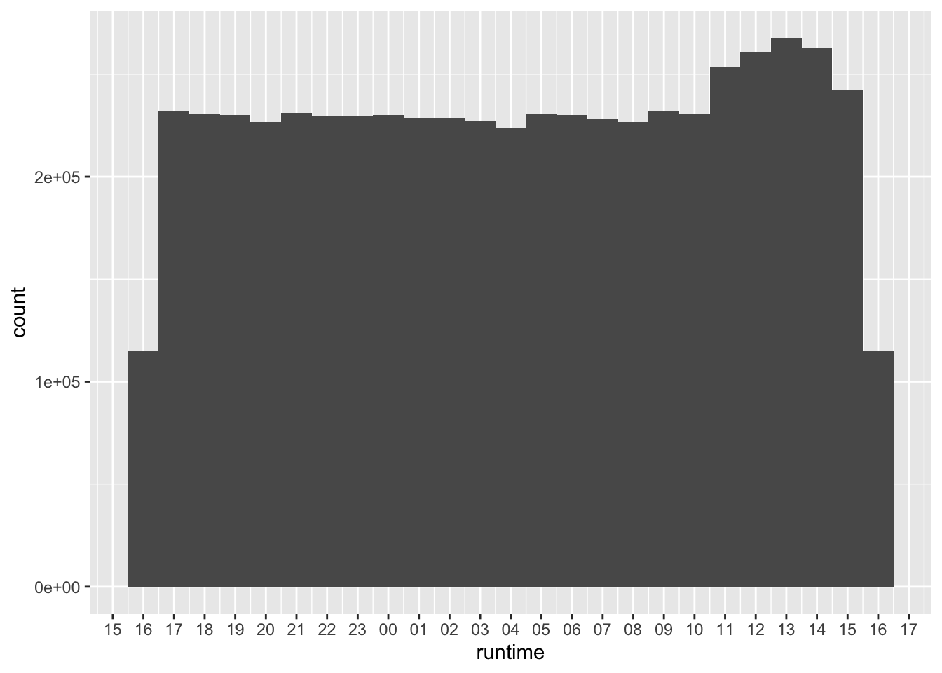

Figure 1: Distribution of times in `runtime`

Footnotes

Execute install.packages(c("tidyverse", duckdb", "tinytable")) within R to install all the packages you need to run the code in this note.↩︎
Some parts of the source code are ugly as I wrangled hurriedly with the output from SQL and LaTeX tables.↩︎
You may need to run INSTALL icu before LOAD icu depending on your DuckDB installation.↩︎

Other Formats

Footnotes